Examples

All notebooks are located at /examples in the OpenOA repository, and can be modified and run on Binder.

Use ENGIE’s open data set

ENGIE provides access to the data of its ‘La Haute Borne’ wind farm through https://opendata-renewables.engie.com and through an API. The data can be used to create additional turbine objects and gives users the opportunity to work with further real-world data.

The series of notebooks in the ‘examples’ folder uses SCADA data downloaded from https://opendata-renewables.engie.com, saved in the ‘examples/data’ folder. Additional plant level meter, availability, and curtailment data were synthesized based on the SCADA data.

In the following example, data is loaded into a turbine object and plotted as a power curve. The selected turbine can be changed if desired.

import matplotlib.pyplot as plt
import numpy as np
import pandas as pd

from bokeh.plotting import show
from bokeh.io import output_notebook
output_notebook()

from project_ENGIE import Project_Engie
from operational_analysis.toolkits import filters
from operational_analysis.toolkits import power_curve
from operational_analysis.toolkits import pandas_plotting

Loading BokehJS ...

Import the data

project = Project_Engie('./data/la_haute_borne')
project.prepare()

INFO:project_ENGIE:Loading SCADA data
INFO:operational_analysis.types.timeseries_table:Loading name:la-haute-borne-data-2014-2015
INFO:project_ENGIE:SCADA data loaded
INFO:project_ENGIE:Timestamp QC and conversion to UTC
INFO:project_ENGIE:Correcting for out of range of temperature variables
INFO:project_ENGIE:Flagging unresponsive sensors
INFO:project_ENGIE:Converting field names to IEC 61400-25 standard
INFO:operational_analysis.types.timeseries_table:Loading name:plant_data
INFO:operational_analysis.types.timeseries_table:Loading name:plant_data
INFO:operational_analysis.types.timeseries_table:Loading name:merra2_la_haute_borne
INFO:operational_analysis.types.timeseries_table:Loading name:era5_wind_la_haute_borne

Now the data is imported we can take a look at the wind farm. There are 4 turbines, nearby foresty, a small town and neighbouring wind farms, which could impact on performance. Now lets have a look at the turbines.

show(pandas_plotting.plot_windfarm(project,tile_name="OpenMap",plot_width=600,plot_height=600))

# List of turbines
turb_list = project.scada.df.id.unique()
turb_list

array(['R80736', 'R80721', 'R80790', 'R80711'], dtype=object)

Let’s examine the first turbine from the list above.

df = project.scada.df.loc[project.scada.df['id'] == turb_list[0]]
windspeed = df["wmet_wdspd_avg"]
power_kw = df["wtur_W_avg"]/1000 # Put into kW

def plot_flagged_pc(ws, p, flag_bool, alpha):
    plt.scatter(ws, p, s = 1, alpha = alpha)
    plt.scatter(ws[flag_bool], p[flag_bool], s = 1, c = 'red')
    plt.xlabel('Wind speed (m/s)')
    plt.ylabel('Power (W)')
    plt.show()

First, we’ll make a scatter plot the raw power curve data.

plot_flagged_pc(windspeed, power_kw, np.repeat(True, df.shape[0]), 1)

Range filter

out_of_range = filters.range_flag(windspeed, below=0, above=70)
windspeed[out_of_range].head()

Series([], Name: wmet_wdspd_avg, dtype: float64)

No wind speeds out of range

Window range filter

Now, we’ll apply a window range filter to remove data with power values outside of the window from 20 to 2100 kW for wind speeds between 5 and 40 m/s.

out_of_window = filters.window_range_flag(windspeed, 5., 40, power_kw, 20., 2100.)
plot_flagged_pc(windspeed, power_kw, out_of_window, 0.2)

Let’s remove these flagged data from consideration

windspeed_filt1 = windspeed[~out_of_window]
power_kw_filt1 = power_kw[~out_of_window]

Bin filter

We may be interested in fitting a power curve to data representing ‘normal’ turbine operation. In other words, we want to flag all anomalous data or data represenatative of underperformance. To do this, the ‘bin_filter’ function is useful. It works by binning the data by a specified variable, bin width, and start and end points. The criteria for flagging is based on some measure (scalar or standard deviation) from the mean or median of the bin center.

As an example, let’s bin on power in 100 kW increments, starting from 25.0 kW but stopping at 90% of peak power (i.e. we don’t want to flag all the data at peak power and high wind speed. Let’s use a scalar threshold of 1.5 m/s from the median for each bin. Let’s also consider data on both sides of the curve by setting the ‘direction’ parameter to ‘all’

max_bin = 0.90*power_kw_filt1.max()
bin_outliers = filters.bin_filter(power_kw_filt1, windspeed_filt1, 100, 1.5, 'median', 20., max_bin, 'scalar', 'all')
plot_flagged_pc(windspeed_filt1, power_kw_filt1, bin_outliers, 0.5)

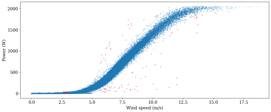
As seen above, one call for the bin filter has done a decent job of cleaning up the power curve to represent ‘normal’ operation, without excessive removal of data points. There are a few points at peak power but low wind speed that weren’t flagged, however. Let catch those, and then remove those as well as the flagged data above, and plot our ‘clean’ power curve

windspeed_filt2 = windspeed_filt1[~bin_outliers]
power_kw_filt2 = power_kw_filt1[~bin_outliers]

Unresponsive Filter

As a final filtering demonstration, we can look for an unrespsonsive sensor (i.e. repeating measurements). In this case, let’s look for 3 or more repeating wind speed measurements:

frozen = filters.unresponsive_flag(windspeed_filt2, 3)
windspeed_filt2[frozen]

time
2014-01-10 14:40:00    0.0
2014-01-10 14:50:00    0.0
2014-01-10 15:00:00    0.0
2014-01-11 22:30:00    0.0
2014-01-11 22:40:00    0.0
                      ...
2015-12-09 22:50:00    0.0
2015-12-09 23:00:00    0.0
2015-12-15 02:20:00    5.5
2015-12-15 02:30:00    5.5
2015-12-15 02:40:00    5.5
Name: wmet_wdspd_avg, Length: 1926, dtype: float64

We actually found a lot, so let’s remove these data as well before moving on to power curve fitting.

Note that many of the unresponsive sensor values identified above are likely caused by the discretization of the data to only two decimal places. However, the goal is to illustrate the filtering process.

windspeed_final = windspeed_filt2[~frozen]
power_kw_final = power_kw_filt2[~frozen]

Power curve fitting

We will now consider three different models for fitting a power curve to the SCADA data.

# Fit the power curves
iec_curve = power_curve.IEC(windspeed_final, power_kw_final)
l5p_curve = power_curve.logistic_5_parametric(windspeed_final, power_kw_final)
spline_curve = power_curve.gam(windspeed_final, power_kw_final, n_splines = 20)

# Plot the results
x = np.linspace(0,20,100)
plt.figure(figsize = (10,6))
plt.scatter(windspeed_final, power_kw_final, alpha=0.5, s = 1, c = 'gray')
plt.plot(x, iec_curve(x), color="red", label = 'IEC', linewidth = 3)
plt.plot(x, spline_curve(x), color="C1", label = 'Spline', linewidth = 3)
plt.plot(x, l5p_curve(x), color="C2", label = 'L5P', linewidth = 3)
plt.xlabel('Wind speed (m/s)')
plt.ylabel('Power (kW)')
plt.legend()
plt.show()

The above plot shows that the IEC method accurately captures the power curve, although it results in a ‘choppy’ fit, while the L5P model (constrained by its parametric form) deviates from the knee of the power curve through peak production. The spline fit tends to fit the best.

Quality Check Diagnostic Work, Part A

This notebook illustrates some quality control steps that should be considered when analyzing a new dataset. In this example we’ll use the WindToolKitQualityControlDiagnosticSuite class to automate some of the QC analysis for SCADA data.

The WindToolKitQualityDiagnosticSuite is a subclass of the QualityControlDiagnosticSuite that adds additional methods for the use of the NREL WindToolKit database in addition to all the base QC methods.

In part A of this exercise, we will demonstrate the use of timezone-naive timestamps.

Step 1: Load in Data

To load in the data, we can either preload the data, or pass in a full file path and have the QC class import the data file.

For this example we’ll load in the data first, and remove the timezone data from the datetime stamp to demonstrate the process of uncovering the DST overlap in the data.

%load_ext autoreload
%autoreload 2

import numpy as np
import pandas as pd

from operational_analysis.methods.quality_check_automation import WindToolKitQualityControlDiagnosticSuite as QC

scada_df = pd.read_csv('./data/la_haute_borne/la-haute-borne-data-2014-2015.csv')

date = [s[0:10] for s in scada_df['Date_time']]
time = [s[11:19] for s in scada_df['Date_time']]
datetime = [date[s] + ' ' + time[s] for s in np.arange(len(date))]
scada_df['datetime'] = pd.to_datetime(datetime, format = "%Y-%m-%d %H:%M:%S")

scada_df.set_index('datetime', inplace = True, drop = False)

scada_df.head()

	Wind_turbine_name	Date_time	Ba_avg	P_avg	Ws_avg	Va_avg	Ot_avg	Ya_avg	Wa_avg	datetime
datetime
2014-01-01 01:00:00	R80736	2014-01-01T01:00:00+01:00	-1.00	642.78003	7.12	0.66	4.69	181.34000	182.00999	2014-01-01 01:00:00
2014-01-01 01:00:00	R80721	2014-01-01T01:00:00+01:00	-1.01	441.06000	6.39	-2.48	4.94	179.82001	177.36000	2014-01-01 01:00:00
2014-01-01 01:00:00	R80790	2014-01-01T01:00:00+01:00	-0.96	658.53003	7.11	1.07	4.55	172.39000	173.50999	2014-01-01 01:00:00
2014-01-01 01:00:00	R80711	2014-01-01T01:00:00+01:00	-0.93	514.23999	6.87	6.95	4.30	172.77000	179.72000	2014-01-01 01:00:00
2014-01-01 01:10:00	R80790	2014-01-01T01:10:00+01:00	-0.96	640.23999	7.01	-1.90	4.68	172.39000	170.46001	2014-01-01 01:10:00

scada_df.dtypes

Wind_turbine_name            object
Date_time                    object
Ba_avg                      float64
P_avg                       float64
Ws_avg                      float64
Va_avg                      float64
Ot_avg                      float64
Ya_avg                      float64
Wa_avg                      float64
datetime             datetime64[ns]
dtype: object

Step 2: Initializing QC and Performing the Run Method

Now that we have our dataset with the necessary columns and datatypes, we are ready to perform our quality check diagnostic. This analysis will not make the adjustments for us, but it will allow us to quickly flag some key irregularities that we need to manage before going on.

To start, let’s initialize a QC object, qc, and call its run method.

qc = QC(
    data=scada_df,
    ws_field='Ws_avg',
    power_field= 'P_avg',
    time_field='datetime',
    id_field='Wind_turbine_name',
    freq='10T',
    lat_lon=(48.45, 5.586),
    # It is highly recommended to add the local timezone even if it may not be present
    local_tz="Europe/Paris",
    timezone_aware=False,  # We should indicate that the timezone in the data is unknown
    check_tz=False,  # True for WIND ToolKit-valid locations only, though will not break the code if outside
)

INFO:operational_analysis.methods.quality_check_automation:Initializing QC_Automation Object

Below is what the updated DataFrame object looks like after being read in and manipulated for the initial setup. Notice that there is now a UTC offset column, which directly translates to the is_dst column’s True/False input for whether or not a particular timestamp is in Daylight Saving’s Time (if it’s used at all for the time zone).

In the below, the datetime_utc column should always remain in UTC time and the datetime_localized column should always remain in the localized time. Conveniently, Pandas provides two methods tz_convert() and tz_localize() to toggle back and forth between timezones, which will operate on the index of the DataFrame. It is worth noting that the local time could also be UTC, in which case the two columns would be redundant.

The localized time, even when the passed data is unaware, is adjusted using the local_tz keyword argument to help normalize the time strings, from which a UTC-based timestamp is created (even when local is also UTC). By calculating the UTC time from the local time, we are able to ascertain DST shifts in the data, and better assess any anomalies that may exist.

However, there may be cases where the timezone is not encoded (this example), nor known. In the former, we can use the local_tz keyword argument that is seen in the code above, but for the latter, this is much more difficult, and the default value of UTC may not be accurate. In this latter case it is useful to try multiple timezones, such as an operating/owner company’s headquarters or often the windfarm’s location to find a best fit. In the case of using a US-based windfarm, the subclass WindToolKitQualityControlDiagnosticSuite can be used to help better match a timezone and the data provided.

qc._df.head()

	Wind_turbine_name	Date_time	Ba_avg	P_avg	Ws_avg	Va_avg	Ot_avg	Ya_avg	Wa_avg	datetime	datetime_localized	datetime_utc	utc_offset	is_dst
datetime_utc
2014-01-01 00:00:00+00:00	R80736	2014-01-01T01:00:00+01:00	-1.00	642.78003	7.12	0.66	4.69	181.34000	182.00999	2014-01-01 01:00:00	2014-01-01 01:00:00+01:00	2014-01-01 00:00:00+00:00	0 days 01:00:00	False
2014-01-01 00:00:00+00:00	R80721	2014-01-01T01:00:00+01:00	-1.01	441.06000	6.39	-2.48	4.94	179.82001	177.36000	2014-01-01 01:00:00	2014-01-01 01:00:00+01:00	2014-01-01 00:00:00+00:00	0 days 01:00:00	False
2014-01-01 00:00:00+00:00	R80790	2014-01-01T01:00:00+01:00	-0.96	658.53003	7.11	1.07	4.55	172.39000	173.50999	2014-01-01 01:00:00	2014-01-01 01:00:00+01:00	2014-01-01 00:00:00+00:00	0 days 01:00:00	False
2014-01-01 00:00:00+00:00	R80711	2014-01-01T01:00:00+01:00	-0.93	514.23999	6.87	6.95	4.30	172.77000	179.72000	2014-01-01 01:00:00	2014-01-01 01:00:00+01:00	2014-01-01 00:00:00+00:00	0 days 01:00:00	False
2014-01-01 00:10:00+00:00	R80790	2014-01-01T01:10:00+01:00	-0.96	640.23999	7.01	-1.90	4.68	172.39000	170.46001	2014-01-01 01:10:00	2014-01-01 01:10:00+01:00	2014-01-01 00:10:00+00:00	0 days 01:00:00	False

qc._df.dtypes

Wind_turbine_name                           object
Date_time                                   object
Ba_avg                                     float64
P_avg                                      float64
Ws_avg                                     float64
Va_avg                                     float64
Ot_avg                                     float64
Ya_avg                                     float64
Wa_avg                                     float64
datetime                            datetime64[ns]
datetime_localized    datetime64[ns, Europe/Paris]
datetime_utc                   datetime64[ns, UTC]
utc_offset                         timedelta64[ns]
is_dst                                        bool
dtype: object

qc.run()

INFO:operational_analysis.methods.quality_check_automation:Identifying Time Duplications
INFO:operational_analysis.methods.quality_check_automation:Identifying Time Gaps
INFO:operational_analysis.methods.quality_check_automation:Isolating Extrema Values
INFO:operational_analysis.methods.quality_check_automation:QC Diagnostic Complete

Step 3: Deep Dive with QC Diagnostic Results

Let’s take a deeper look at the results of our QC diagnostic.

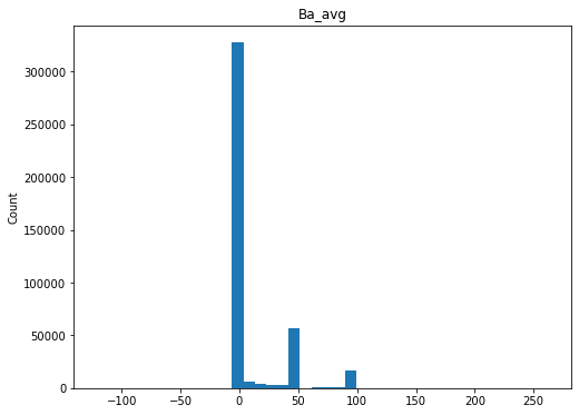
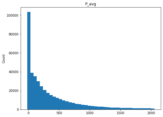
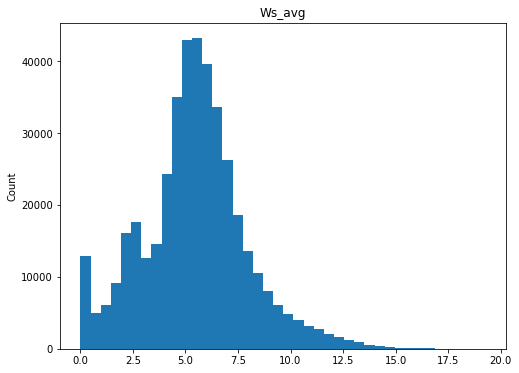
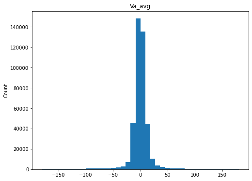
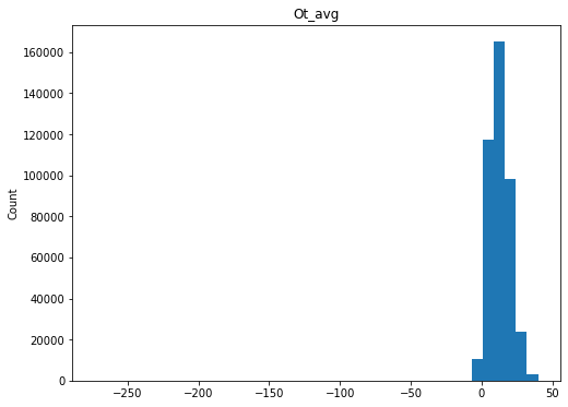
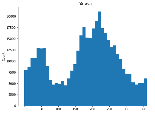
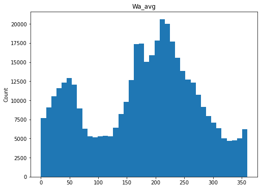
Perform a general scan of the distributions for each numeric variable

qc.column_histograms()

Check ranges of each variable

qc._max_min

	max	min
Wind_turbine_name	R80790	R80711
Date_time	2016-01-01T00:50:00+01:00	2014-01-01T01:00:00+01:00
Ba_avg	262.61	-121.26
P_avg	2051.87	-17.92
Ws_avg	19.31	0
Va_avg	179.99	-179.95
Ot_avg	39.89	-273.2
Ya_avg	360	0
Wa_avg	360	0
datetime	2016-01-01 00:50:00	2014-01-01 01:00:00
datetime_localized	2016-01-01 00:50:00+01:00	2014-01-01 01:00:00+01:00
datetime_utc	2015-12-31 23:50:00+00:00	2014-01-01 00:00:00+00:00
utc_offset	0 days 02:00:00	0 days 01:00:00
is_dst	True	False

These values look fairly reasonable and consistent.

Identify any timestamp duplications and timestamp gaps.

Duplications in October and gaps in March would suggest DST.

qc._time_duplications

datetime_utc
2014-03-30 01:00:00+00:00   2014-03-30 03:00:00
2014-03-30 01:00:00+00:00   2014-03-30 03:00:00
2014-03-30 01:00:00+00:00   2014-03-30 03:00:00
2014-03-30 01:00:00+00:00   2014-03-30 03:00:00
2014-03-30 01:10:00+00:00   2014-03-30 03:10:00
2014-03-30 01:10:00+00:00   2014-03-30 03:10:00
2014-03-30 01:10:00+00:00   2014-03-30 03:10:00
2014-03-30 01:10:00+00:00   2014-03-30 03:10:00
2014-03-30 01:20:00+00:00   2014-03-30 03:20:00
2014-03-30 01:20:00+00:00   2014-03-30 03:20:00
2014-03-30 01:20:00+00:00   2014-03-30 03:20:00
2014-03-30 01:20:00+00:00   2014-03-30 03:20:00
2014-03-30 01:30:00+00:00   2014-03-30 03:30:00
2014-03-30 01:30:00+00:00   2014-03-30 03:30:00
2014-03-30 01:30:00+00:00   2014-03-30 03:30:00
2014-03-30 01:30:00+00:00   2014-03-30 03:30:00
2014-03-30 01:40:00+00:00   2014-03-30 03:40:00
2014-03-30 01:40:00+00:00   2014-03-30 03:40:00
2014-03-30 01:40:00+00:00   2014-03-30 03:40:00
2014-03-30 01:40:00+00:00   2014-03-30 03:40:00
2014-03-30 01:50:00+00:00   2014-03-30 03:50:00
2014-03-30 01:50:00+00:00   2014-03-30 03:50:00
2014-03-30 01:50:00+00:00   2014-03-30 03:50:00
2014-03-30 01:50:00+00:00   2014-03-30 03:50:00
2015-03-29 01:00:00+00:00   2015-03-29 03:00:00
2015-03-29 01:00:00+00:00   2015-03-29 03:00:00
2015-03-29 01:00:00+00:00   2015-03-29 03:00:00
2015-03-29 01:00:00+00:00   2015-03-29 03:00:00
2015-03-29 01:10:00+00:00   2015-03-29 03:10:00
2015-03-29 01:10:00+00:00   2015-03-29 03:10:00
2015-03-29 01:10:00+00:00   2015-03-29 03:10:00
2015-03-29 01:10:00+00:00   2015-03-29 03:10:00
2015-03-29 01:20:00+00:00   2015-03-29 03:20:00
2015-03-29 01:20:00+00:00   2015-03-29 03:20:00
2015-03-29 01:20:00+00:00   2015-03-29 03:20:00
2015-03-29 01:20:00+00:00   2015-03-29 03:20:00
2015-03-29 01:30:00+00:00   2015-03-29 03:30:00
2015-03-29 01:30:00+00:00   2015-03-29 03:30:00
2015-03-29 01:30:00+00:00   2015-03-29 03:30:00
2015-03-29 01:30:00+00:00   2015-03-29 03:30:00
2015-03-29 01:40:00+00:00   2015-03-29 03:40:00
2015-03-29 01:40:00+00:00   2015-03-29 03:40:00
2015-03-29 01:40:00+00:00   2015-03-29 03:40:00
2015-03-29 01:40:00+00:00   2015-03-29 03:40:00
2015-03-29 01:50:00+00:00   2015-03-29 03:50:00
2015-03-29 01:50:00+00:00   2015-03-29 03:50:00
2015-03-29 01:50:00+00:00   2015-03-29 03:50:00
2015-03-29 01:50:00+00:00   2015-03-29 03:50:00
Name: datetime, dtype: datetime64[ns]

qc._time_duplications_utc

datetime_utc
2014-03-30 01:00:00+00:00   2014-03-30 01:00:00+00:00
2014-03-30 01:00:00+00:00   2014-03-30 01:00:00+00:00
2014-03-30 01:00:00+00:00   2014-03-30 01:00:00+00:00
2014-03-30 01:00:00+00:00   2014-03-30 01:00:00+00:00
2014-03-30 01:10:00+00:00   2014-03-30 01:10:00+00:00
2014-03-30 01:10:00+00:00   2014-03-30 01:10:00+00:00
2014-03-30 01:10:00+00:00   2014-03-30 01:10:00+00:00
2014-03-30 01:10:00+00:00   2014-03-30 01:10:00+00:00
2014-03-30 01:20:00+00:00   2014-03-30 01:20:00+00:00
2014-03-30 01:20:00+00:00   2014-03-30 01:20:00+00:00
2014-03-30 01:20:00+00:00   2014-03-30 01:20:00+00:00
2014-03-30 01:20:00+00:00   2014-03-30 01:20:00+00:00
2014-03-30 01:30:00+00:00   2014-03-30 01:30:00+00:00
2014-03-30 01:30:00+00:00   2014-03-30 01:30:00+00:00
2014-03-30 01:30:00+00:00   2014-03-30 01:30:00+00:00
2014-03-30 01:30:00+00:00   2014-03-30 01:30:00+00:00
2014-03-30 01:40:00+00:00   2014-03-30 01:40:00+00:00
2014-03-30 01:40:00+00:00   2014-03-30 01:40:00+00:00
2014-03-30 01:40:00+00:00   2014-03-30 01:40:00+00:00
2014-03-30 01:40:00+00:00   2014-03-30 01:40:00+00:00
2014-03-30 01:50:00+00:00   2014-03-30 01:50:00+00:00
2014-03-30 01:50:00+00:00   2014-03-30 01:50:00+00:00
2014-03-30 01:50:00+00:00   2014-03-30 01:50:00+00:00
2014-03-30 01:50:00+00:00   2014-03-30 01:50:00+00:00
2015-03-29 01:00:00+00:00   2015-03-29 01:00:00+00:00
2015-03-29 01:00:00+00:00   2015-03-29 01:00:00+00:00
2015-03-29 01:00:00+00:00   2015-03-29 01:00:00+00:00
2015-03-29 01:00:00+00:00   2015-03-29 01:00:00+00:00
2015-03-29 01:10:00+00:00   2015-03-29 01:10:00+00:00
2015-03-29 01:10:00+00:00   2015-03-29 01:10:00+00:00
2015-03-29 01:10:00+00:00   2015-03-29 01:10:00+00:00
2015-03-29 01:10:00+00:00   2015-03-29 01:10:00+00:00
2015-03-29 01:20:00+00:00   2015-03-29 01:20:00+00:00
2015-03-29 01:20:00+00:00   2015-03-29 01:20:00+00:00
2015-03-29 01:20:00+00:00   2015-03-29 01:20:00+00:00
2015-03-29 01:20:00+00:00   2015-03-29 01:20:00+00:00
2015-03-29 01:30:00+00:00   2015-03-29 01:30:00+00:00
2015-03-29 01:30:00+00:00   2015-03-29 01:30:00+00:00
2015-03-29 01:30:00+00:00   2015-03-29 01:30:00+00:00
2015-03-29 01:30:00+00:00   2015-03-29 01:30:00+00:00
2015-03-29 01:40:00+00:00   2015-03-29 01:40:00+00:00
2015-03-29 01:40:00+00:00   2015-03-29 01:40:00+00:00
2015-03-29 01:40:00+00:00   2015-03-29 01:40:00+00:00
2015-03-29 01:40:00+00:00   2015-03-29 01:40:00+00:00
2015-03-29 01:50:00+00:00   2015-03-29 01:50:00+00:00
2015-03-29 01:50:00+00:00   2015-03-29 01:50:00+00:00
2015-03-29 01:50:00+00:00   2015-03-29 01:50:00+00:00
2015-03-29 01:50:00+00:00   2015-03-29 01:50:00+00:00
Name: datetime_utc, dtype: datetime64[ns, UTC]

qc._time_gaps

12678   2014-03-30 02:00:00
12679   2014-03-30 02:10:00
12680   2014-03-30 02:20:00
12681   2014-03-30 02:30:00
12682   2014-03-30 02:40:00
12683   2014-03-30 02:50:00
65094   2015-03-29 02:00:00
65095   2015-03-29 02:10:00
65096   2015-03-29 02:20:00
65097   2015-03-29 02:30:00
65098   2015-03-29 02:40:00
65099   2015-03-29 02:50:00
dtype: datetime64[ns]

qc._time_gaps_utc

42918   2014-10-26 01:00:00+00:00
42919   2014-10-26 01:10:00+00:00
42920   2014-10-26 01:20:00+00:00
42921   2014-10-26 01:30:00+00:00
42922   2014-10-26 01:40:00+00:00
42923   2014-10-26 01:50:00+00:00
95334   2015-10-25 01:00:00+00:00
95335   2015-10-25 01:10:00+00:00
95336   2015-10-25 01:20:00+00:00
95337   2015-10-25 01:30:00+00:00
95338   2015-10-25 01:40:00+00:00
95339   2015-10-25 01:50:00+00:00
dtype: datetime64[ns, UTC]

Based on the duplicated timestamps, it does seem like there is a DST correction in spring but no duplicate times in the fall. However, even with a UTC conversion, there still appear to be duplications in the data, so there is likely additional analysis needed here. While it appears that there are time gaps in the data for the original inputs, this phenomena switches seasons to the fall for the UTC converted time stamps, likely due to the lack of timezone encoding in the original inputs compared to a corrected timestamp.

Check the DST plot to look in more detail

qc.daylight_savings_plot()

It appears that the original data (blue, solid line, labeled “Original Timestamp”) has a time gap in the spring; however, when we compare it to the UTC timestamp (orange, dashed line), it is clear that there is not in fact any gap in the data, and the DST transition has been encoded properly in the data. On the otherhand, it at first appears that there are no gaps in the fall when we make the same comparison, but when looking at the UTC timestamps, we can see that there is a 1 hour gap in the data for both 2014 and 2015. This is in line with our comparison of qc._time_gaps and qc._time_gaps_utc above, and further confirms our findings that there are duplicates in the spring and gaps in the fall.

By having the original data and a UTC-converted timestamp it enables us to see any gaps that may appear when there is no timezone data encoded. On the other hand, using the UTC-converted timestamp does not reduce the number of duplications in this dataset that are present in the spring, but helps adjust for seemingly missing or available data. In tandem we can see in the scatter points that there are still duplicates in the spring data just before the

The final question regarding datetime is whether we’re in UTC or local. Given the daylights savings gap, it’s likely we’re in local. This is further confirmed by the raw datetime info provided in the SCADA file, which shows either a +1h or +2h timezone from UTC. So we are operating in local time. Therefore, the project import script for La Haute Borne should shift the timestep back to put it into UTC.

Inspect the turbine power curves

Now that we have gathered some useful information about our timeseries, the one last check we may want to make is to inspect each turbine profile. We can look at each turbine’s power curve and perform an initial scan for irregularities.

qc.plot_by_id('Ws_avg', 'P_avg')

/Users/rhammond/Documents/GitHub/OpenOA/operational_analysis/methods/quality_check_automation.py:488: MatplotlibDeprecationWarning: Passing non-integers as three-element position specification is deprecated since 3.3 and will be removed two minor releases later.
  plt.subplot(num_rows, 4, n)

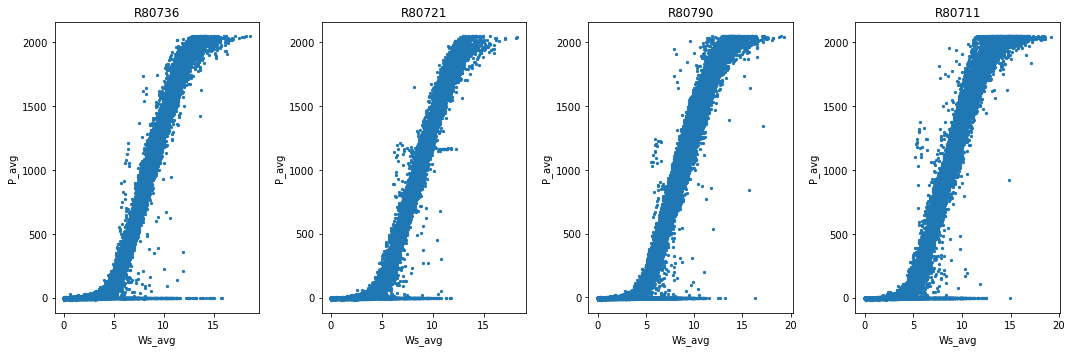
Overall, these power curves look pretty common with some downtime, derating, and what look like a few erroneous data points.

Step 4: Performing adjustments on our data

Recall that this notebook is only for diagnostic QC of plant data and does not actually change the data in the project import script. Any issues identifed here should be incorporated into the project import script.

Note that the necessary corrections have already been applied to the project import script for this data.

Quality Check Diagnostic Work, Part B

This notebook illustrates some quality control steps that should be considered when analyzing a new dataset. In this example we’ll use the WindToolKitQualityControlDiagnosticSuite class to automate some of the QC analysis for SCADA data.

The WindToolKitQualityDiagnosticSuite is a subclass of the QualityControlDiagnosticSuite that adds additional methods for the use of the NREL WindToolKit database in addition to all the base QC methods.

In Part B of this exercise, we will demonstrate the use of timezone-aware timestamps.

Step 1: Load in Data

To load in the data, we can either preload the data, or pass in a full file path and have the QC class import the data file. We’ll import the data first to give a glimpse into what the data look like.

%load_ext autoreload
%autoreload 2

import numpy as np
import pandas as pd

from operational_analysis.methods.quality_check_automation import WindToolKitQualityControlDiagnosticSuite as QC

scada_df = pd.read_csv('./data/la_haute_borne/la-haute-borne-data-2014-2015.csv')

scada_df.head()

	Wind_turbine_name	Date_time	Ba_avg	P_avg	Ws_avg	Va_avg	Ot_avg	Ya_avg	Wa_avg
0	R80736	2014-01-01T01:00:00+01:00	-1.00	642.78003	7.12	0.66	4.69	181.34000	182.00999
1	R80721	2014-01-01T01:00:00+01:00	-1.01	441.06000	6.39	-2.48	4.94	179.82001	177.36000
2	R80790	2014-01-01T01:00:00+01:00	-0.96	658.53003	7.11	1.07	4.55	172.39000	173.50999
3	R80711	2014-01-01T01:00:00+01:00	-0.93	514.23999	6.87	6.95	4.30	172.77000	179.72000
4	R80790	2014-01-01T01:10:00+01:00	-0.96	640.23999	7.01	-1.90	4.68	172.39000	170.46001

Step 2: Initializing QC and Performing the Run Method

Now that we have our dataset with the necessary columns and datatypes, we are ready to perform our quality check diagnostic. This analysis will not make the adjustments for us, but it will allow us to quickly flag some key irregularities that we need to manage before going on.

To start, let’s initialize a QC object, qc, and call its run method.

qc = QC(
    data=scada_df,
    ws_field='Ws_avg',
    power_field= 'P_avg',
    time_field='Date_time',
    id_field='Wind_turbine_name',
    freq='10T',
    lat_lon=(48.45, 5.586),
    local_tz="Europe/Paris",  # While it may already be present in the timestamps, this should be used!
    timezone_aware=True,  # We should indicate that the timezone in the data is known
    check_tz=False,  # True for WIND ToolKit-valid locations only, though will not break the code if outside
)

INFO:operational_analysis.methods.quality_check_automation:Initializing QC_Automation Object

Below is what the updated DataFrame object looks like after being read in and manipulated for the initial setup. Notice that there is now a UTC offset column, which directly translates to the is_dst column’s True/False input for whether or not a particular timestamp is in Daylight Saving’s Time (if it’s used at all for the time zone).

In the below, the Date_time_UTC column should always remain in UTC time and the Date_time_localized column should always remain in the localized time. Conveniently, Pandas provides two methods tz_convert() and tz_localize() to toggle back and forth between timezones, which will operate on the index of the DataFrame. It is worth noting that the local time could also be UTC, in which case the two columns would be redundant.

The localized time, even when the passed data is unaware, is adjusted using the local_tz keyword argument to help normalize the time strings, from which a UTC-based timestamp is created (even when local is also UTC). By calculating the UTC time from the local time, we are able to ascertain DST shifts in the data, and better assess any anomalies that may exist.

qc._df.head()

	Wind_turbine_name	Date_time	Ba_avg	P_avg	Ws_avg	Va_avg	Ot_avg	Ya_avg	Wa_avg	Date_time_localized	Date_time_utc	utc_offset	is_dst
Date_time_utc
2014-01-01 00:00:00+00:00	R80736	2014-01-01 01:00:00+01:00	-1.00	642.78003	7.12	0.66	4.69	181.34000	182.00999	2014-01-01 01:00:00+01:00	2014-01-01 00:00:00+00:00	0 days 01:00:00	False
2014-01-01 00:00:00+00:00	R80721	2014-01-01 01:00:00+01:00	-1.01	441.06000	6.39	-2.48	4.94	179.82001	177.36000	2014-01-01 01:00:00+01:00	2014-01-01 00:00:00+00:00	0 days 01:00:00	False
2014-01-01 00:00:00+00:00	R80790	2014-01-01 01:00:00+01:00	-0.96	658.53003	7.11	1.07	4.55	172.39000	173.50999	2014-01-01 01:00:00+01:00	2014-01-01 00:00:00+00:00	0 days 01:00:00	False
2014-01-01 00:00:00+00:00	R80711	2014-01-01 01:00:00+01:00	-0.93	514.23999	6.87	6.95	4.30	172.77000	179.72000	2014-01-01 01:00:00+01:00	2014-01-01 00:00:00+00:00	0 days 01:00:00	False
2014-01-01 00:10:00+00:00	R80790	2014-01-01 01:10:00+01:00	-0.96	640.23999	7.01	-1.90	4.68	172.39000	170.46001	2014-01-01 01:10:00+01:00	2014-01-01 00:10:00+00:00	0 days 01:00:00	False

qc._df.dtypes

Wind_turbine_name                            object
Date_time              datetime64[ns, Europe/Paris]
Ba_avg                                      float64
P_avg                                       float64
Ws_avg                                      float64
Va_avg                                      float64
Ot_avg                                      float64
Ya_avg                                      float64
Wa_avg                                      float64
Date_time_localized    datetime64[ns, Europe/Paris]
Date_time_utc                   datetime64[ns, UTC]
utc_offset                          timedelta64[ns]
is_dst                                         bool
dtype: object

qc.run()

INFO:operational_analysis.methods.quality_check_automation:Identifying Time Duplications
INFO:operational_analysis.methods.quality_check_automation:Identifying Time Gaps
INFO:operational_analysis.methods.quality_check_automation:Isolating Extrema Values
INFO:operational_analysis.methods.quality_check_automation:QC Diagnostic Complete

Step 3: Deep Dive with QC Diagnostic Results

Let’s take a deeper look at the results of our QC diagnostic.

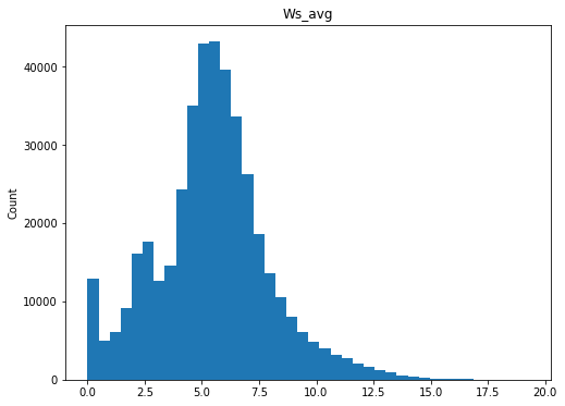
Perform a general scan of the distributions for each numeric variable

qc.column_histograms()

Check ranges of each variable

qc._max_min

	min	max
Wind_turbine_name	R80711	R80790
Date_time	2014-01-01 01:00:00+01:00	2016-01-01 00:50:00+01:00
Ba_avg	-121.26	262.61
P_avg	-17.92	2051.87
Ws_avg	0	19.31
Va_avg	-179.95	179.99
Ot_avg	-273.2	39.89
Ya_avg	0	360
Wa_avg	0	360
Date_time_localized	2014-01-01 01:00:00+01:00	2016-01-01 00:50:00+01:00
Date_time_utc	2014-01-01 00:00:00+00:00	2015-12-31 23:50:00+00:00
utc_offset	0 days 01:00:00	0 days 02:00:00
is_dst	False	True

These values look fairly reasonable and consistent.

Identify any timestamp duplications and timestamp gaps.

Duplications in October and gaps in March would suggest DST.

qc._time_duplications

Date_time_utc
2014-03-30 01:00:00+00:00   2014-03-30 03:00:00+02:00
2014-03-30 01:00:00+00:00   2014-03-30 03:00:00+02:00
2014-03-30 01:00:00+00:00   2014-03-30 03:00:00+02:00
2014-03-30 01:00:00+00:00   2014-03-30 03:00:00+02:00
2014-03-30 01:10:00+00:00   2014-03-30 03:10:00+02:00
2014-03-30 01:10:00+00:00   2014-03-30 03:10:00+02:00
2014-03-30 01:10:00+00:00   2014-03-30 03:10:00+02:00
2014-03-30 01:10:00+00:00   2014-03-30 03:10:00+02:00
2014-03-30 01:20:00+00:00   2014-03-30 03:20:00+02:00
2014-03-30 01:20:00+00:00   2014-03-30 03:20:00+02:00
2014-03-30 01:20:00+00:00   2014-03-30 03:20:00+02:00
2014-03-30 01:20:00+00:00   2014-03-30 03:20:00+02:00
2014-03-30 01:30:00+00:00   2014-03-30 03:30:00+02:00
2014-03-30 01:30:00+00:00   2014-03-30 03:30:00+02:00
2014-03-30 01:30:00+00:00   2014-03-30 03:30:00+02:00
2014-03-30 01:30:00+00:00   2014-03-30 03:30:00+02:00
2014-03-30 01:40:00+00:00   2014-03-30 03:40:00+02:00
2014-03-30 01:40:00+00:00   2014-03-30 03:40:00+02:00
2014-03-30 01:40:00+00:00   2014-03-30 03:40:00+02:00
2014-03-30 01:40:00+00:00   2014-03-30 03:40:00+02:00
2014-03-30 01:50:00+00:00   2014-03-30 03:50:00+02:00
2014-03-30 01:50:00+00:00   2014-03-30 03:50:00+02:00
2014-03-30 01:50:00+00:00   2014-03-30 03:50:00+02:00
2014-03-30 01:50:00+00:00   2014-03-30 03:50:00+02:00
2015-03-29 01:00:00+00:00   2015-03-29 03:00:00+02:00
2015-03-29 01:00:00+00:00   2015-03-29 03:00:00+02:00
2015-03-29 01:00:00+00:00   2015-03-29 03:00:00+02:00
2015-03-29 01:00:00+00:00   2015-03-29 03:00:00+02:00
2015-03-29 01:10:00+00:00   2015-03-29 03:10:00+02:00
2015-03-29 01:10:00+00:00   2015-03-29 03:10:00+02:00
2015-03-29 01:10:00+00:00   2015-03-29 03:10:00+02:00
2015-03-29 01:10:00+00:00   2015-03-29 03:10:00+02:00
2015-03-29 01:20:00+00:00   2015-03-29 03:20:00+02:00
2015-03-29 01:20:00+00:00   2015-03-29 03:20:00+02:00
2015-03-29 01:20:00+00:00   2015-03-29 03:20:00+02:00
2015-03-29 01:20:00+00:00   2015-03-29 03:20:00+02:00
2015-03-29 01:30:00+00:00   2015-03-29 03:30:00+02:00
2015-03-29 01:30:00+00:00   2015-03-29 03:30:00+02:00
2015-03-29 01:30:00+00:00   2015-03-29 03:30:00+02:00
2015-03-29 01:30:00+00:00   2015-03-29 03:30:00+02:00
2015-03-29 01:40:00+00:00   2015-03-29 03:40:00+02:00
2015-03-29 01:40:00+00:00   2015-03-29 03:40:00+02:00
2015-03-29 01:40:00+00:00   2015-03-29 03:40:00+02:00
2015-03-29 01:40:00+00:00   2015-03-29 03:40:00+02:00
2015-03-29 01:50:00+00:00   2015-03-29 03:50:00+02:00
2015-03-29 01:50:00+00:00   2015-03-29 03:50:00+02:00
2015-03-29 01:50:00+00:00   2015-03-29 03:50:00+02:00
2015-03-29 01:50:00+00:00   2015-03-29 03:50:00+02:00
Name: Date_time, dtype: datetime64[ns, Europe/Paris]

qc._time_gaps

42912   2014-10-26 02:00:00+02:00
42913   2014-10-26 02:10:00+02:00
42914   2014-10-26 02:20:00+02:00
42915   2014-10-26 02:30:00+02:00
42916   2014-10-26 02:40:00+02:00
42917   2014-10-26 02:50:00+02:00
95328   2015-10-25 02:00:00+02:00
95329   2015-10-25 02:10:00+02:00
95330   2015-10-25 02:20:00+02:00
95331   2015-10-25 02:30:00+02:00
95332   2015-10-25 02:40:00+02:00
95333   2015-10-25 02:50:00+02:00
dtype: datetime64[ns, Europe/Paris]

qc._time_gaps_utc

42912   2014-10-26 00:00:00+00:00
42913   2014-10-26 00:10:00+00:00
42914   2014-10-26 00:20:00+00:00
42915   2014-10-26 00:30:00+00:00
42916   2014-10-26 00:40:00+00:00
42917   2014-10-26 00:50:00+00:00
95328   2015-10-25 00:00:00+00:00
95329   2015-10-25 00:10:00+00:00
95330   2015-10-25 00:20:00+00:00
95331   2015-10-25 00:30:00+00:00
95332   2015-10-25 00:40:00+00:00
95333   2015-10-25 00:50:00+00:00
dtype: datetime64[ns, UTC]

Based on the duplicated timestamps, it does seem like there is a DST correction in spring and a time gap in the fall. This is in contrast with Part A of this example where we found gaps in the spring and none in the fall for the original data, and vice versa for the UTC data. The effect is consistent here because the timezone data is now encoded in the data we are working with, and so the DST shifts are encoded accurately, therefore correctly identifying the fall time gaps that were seen in Part A and in the plots below.

Check the DST plot to look in more detail

qc.daylight_savings_plot()

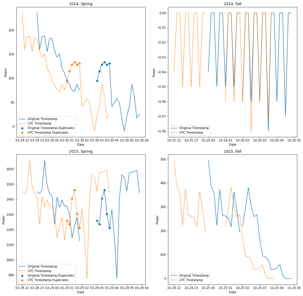
It should be noted that we are able to observe the same phenomena in Part A of this tutorial, which is expected given that it is the same data, but here we already have the timezone encoded within the timestamps, and so are able to confirm that the gaps present in the data are due to the DST transition.

However, we find that the the timing of the transition and therefore the resulting plots has shifted an hour in the fall due to an accurate encoding of the DST transition instead of the implicit encoding from Part A of this example.

Inspect the turbine power curves

Now that we have gathered some useful information about our timeseries, the one last check we may want to make is to inspect each turbine profile. We can look at each turbine’s power curve and perform an initial scan for irregularities.

qc.plot_by_id('Ws_avg', 'P_avg')

/Users/rhammond/Documents/GitHub/OpenOA/operational_analysis/methods/quality_check_automation.py:488: MatplotlibDeprecationWarning: Passing non-integers as three-element position specification is deprecated since 3.3 and will be removed two minor releases later.
  plt.subplot(num_rows, 4, n)

Overall, these power curves look pretty common with some downtime, derating, and what look like a few erroneous data points.

Step 4: Performing adjustments on our data

Recall that this notebook is only for diagnostic QC of plant data and does not actually change the data in the project import script. Any issues identifed here should be incorporated into the project import script.

Note that the necessary corrections have already been applied to the project import script for this data.

First step in gap analysis is to determine the AEP based on operational data.

%load_ext autoreload
%autoreload 2

This notebook provides an overview and walk-through of the steps taken to produce a plant-level operational energy asssessment (OA) of a wind plant in the PRUF project. The La Haute-Borne wind farm is used here and throughout the example notebooks.

Uncertainty in the annual energy production (AEP) estimate is calculated through a Monte Carlo approach. Specifically, inputs into the OA code as well as intermediate calculations are randomly sampled based on their specified or calculated uncertainties. By performing the OA assessment thousands of times under different combinations of the random sampling, a distribution of AEP values results from which uncertainty can be deduced. Details on the Monte Carlo approach will be provided throughout this notebook.

Step 1: Import plant data into notebook

A zip file included in the OpenOA ‘examples/data’ folder needs to be unzipped to run this step. Note that this zip file should be unzipped automatically as part of the project.prepare() function call below. Once unzipped, 4 CSV files will appear in the ‘examples/data/la_haute_borne’ folder.

import os
import matplotlib.pyplot as plt
import numpy as np
import statsmodels.api as sm
import pandas as pd
import copy

from project_ENGIE import Project_Engie
from operational_analysis.methods import plant_analysis

In the call below, make sure the appropriate path to the CSV input files is specfied. In this example, the CSV files are located directly in the ‘examples/data/la_haute_borne’ folder

# Load plant object
project = Project_Engie('./data/la_haute_borne')

# Prepare data
project.prepare()

INFO:project_ENGIE:Loading SCADA data
INFO:operational_analysis.types.timeseries_table:Loading name:la-haute-borne-data-2014-2015
INFO:project_ENGIE:SCADA data loaded
INFO:project_ENGIE:Timestamp QC and conversion to UTC
INFO:project_ENGIE:Correcting for out of range of temperature variables
INFO:project_ENGIE:Flagging unresponsive sensors
INFO:project_ENGIE:Converting field names to IEC 61400-25 standard
INFO:operational_analysis.types.timeseries_table:Loading name:plant_data
INFO:operational_analysis.types.timeseries_table:Loading name:plant_data
INFO:operational_analysis.types.timeseries_table:Loading name:merra2_la_haute_borne
INFO:operational_analysis.types.timeseries_table:Loading name:era5_wind_la_haute_borne

Step 2: Review the data

Several Pandas data frames have now been loaded. Histograms showing the distribution of the plant-level metered energy, availability, and curtailment are shown below:

# Review plant data
fig, (ax1, ax2, ax3) = plt.subplots(ncols = 3, figsize = (15,5))
ax1.hist(project._meter.df['energy_kwh'], 40) # Metered energy data
ax2.hist(project._curtail.df['availability_kwh'], 40) # Curtailment and availability loss data
ax3.hist(project._curtail.df['curtailment_kwh'], 40) # Curtailment and availability loss data
plt.tight_layout()
plt.show()

Step 3: Process the data into monthly averages and sums

The raw plant data can be in different time resolutions (in this case 10-minute periods). The following steps process the data into monthly averages and combine them into a single ‘monthly’ data frame to be used in the OA assessment.

project._meter.df.head()

	energy_kwh	time
time
2014-01-01 00:00:00	369.726	2014-01-01 00:00:00
2014-01-01 00:10:00	376.409	2014-01-01 00:10:00
2014-01-01 00:20:00	309.199	2014-01-01 00:20:00
2014-01-01 00:30:00	350.176	2014-01-01 00:30:00
2014-01-01 00:40:00	286.333	2014-01-01 00:40:00

First, we’ll create a MonteCarloAEP object which is used to calculate long-term AEP. Two renalaysis products are specified as arguments.

pa = plant_analysis.MonteCarloAEP(project, reanal_products = ['era5', 'merra2'])

INFO:operational_analysis.methods.plant_analysis:Initializing MonteCarloAEP Analysis Object

Let’s view the result. Note the extra fields we’ve calculated that we’ll use later for filtering: - energy_nan_perc : the percentage of NaN values in the raw revenue meter data used in calculating the monthly sum. If this value is too large, we shouldn’t include this month - nan_flag : if too much energy, availability, or curtailment data was missing for a given month, flag the result - num_days_expected : number of days in the month (useful for normalizing monthly gross energy later) - num_days_actual : actual number of days per month as found in the data (used when trimming monthly data frame)

# View the monthly data frame
pa._aggregate.df.head()

	energy_gwh	energy_nan_perc	num_days_expected	num_days_actual	availability_gwh	curtailment_gwh	gross_energy_gwh	availability_pct	curtailment_pct	avail_nan_perc	curt_nan_perc	nan_flag	availability_typical	curtailment_typical	combined_loss_valid	era5	merra2
time
2014-01-01	1.279667	0.0	31	31	0.008721	0.000000	1.288387	0.006769	0.000000	0.0	0.0	False	True	True	True	7.314878	7.227947
2014-02-01	1.793873	0.0	28	28	0.005280	0.000000	1.799153	0.002934	0.000000	0.0	0.0	False	True	True	True	8.347006	8.598686
2014-03-01	0.805549	0.0	31	31	0.000151	0.000000	0.805700	0.000188	0.000000	0.0	0.0	False	True	True	True	5.169673	5.207071
2014-04-01	0.636472	0.0	30	30	0.002773	0.000000	0.639245	0.004338	0.000000	0.0	0.0	False	True	True	True	4.756275	4.872304
2014-05-01	1.154255	0.0	31	31	0.015176	0.000225	1.169656	0.012974	0.000192	0.0	0.0	False	True	True	True	6.162751	6.351635

Step 4: Review reanalysis data

Reanalysis data will be used to long-term correct the operational energy over the plant period of operation to the long-term. It is important that we only use reanalysis data that show reasonable trends over time with no noticeable discontinuities. A plot like below, in which normalized annual wind speeds are shown from 1997 to present, provides a good first look at data quality.

The plot shows that both of the reanalysis products track each other reasonably well and seem well-suited for the analysis.

pa.plot_reanalysis_normalized_rolling_monthly_windspeed().show()

Step 5: Review energy and loss data

It is useful to take a look at the energy data and make sure the values make sense. We begin with scatter plots of gross energy and wind speed for each reanalysis product. We also show a time series of gross energy, as well as availability and curtailment loss.

Let’s start with the scatter plots of gross energy vs wind speed for each reanalysis product. Here we use the ‘Robust Linear Model’ (RLM) module of the Statsmodels package with the default Huber algorithm to produce a regression fit that excludes outliers. Data points in red show the outliers, and were excluded based on a Huber sensitivity factor of 3.0.

The plots below reveal that: - there are some outliers - Both renalysis products are strongly correlated with plant energy

If the user would like the RLM outlier detection algorithm to be used in the Monte Carlo analysis, the “outlier_detection” parameter should be set to “True” when calling the plant_analysis class.

pa.plot_reanalysis_gross_energy_data(outlier_thres=3).show()

Next we show time series plots of the monthly gross energy, availabilty, and curtialment. Note that the availability and curtailment data were estimated based on SCADA data from the plant.

Long-term availability and curtailment losses for the plant are calculated based on average percentage losses for each calendar month. Summing those average values weighted by the fraction of long-term gross energy generated in each month yields the long-term annual estimates. Weighting by monthly long-term gross energy helps account for potential correlation between losses and energy production (e.g., high availability losses in summer months with lower energy production). The long-term losses are calculated in Step 9.

pa.plot_aggregate_plant_data_timeseries().show()

Step 6: Specify availabilty and curtailment data not represenative of actual plant performance

There may be anomalies in the reported availabilty that shouldn’t be considered representative of actual plant performance. Force majeure events (e.g. lightning) are a good example. Such losses aren’t typically considered in pre-construction AEP estimates; therefore, plant availablity loss reported in an operational AEP analysis should also not include such losses.

The ‘availability_typical’ and ‘curtailment_typical’ fields in the monthly data frame are initially set to True. Below, individual months can be set to ‘False’ if it is deemed those months are unrepresentative of long-term plant losses. By flagging these months as false, they will be omitted when assessing average availabilty and curtailment loss for the plant.

Justification for removing months from assessing average availabilty or curtailment should come from conversations with the owner/operator. For example, if a high-loss month is found, reasons for the high loss should be discussed with the owner/operator to determine if those losses can be considered representative of average plant operation.

# For illustrative purposes, let's suppose a few months aren't representative of long-term losses
pa._aggregate.df.loc['2014-11-01',['availability_typical','curtailment_typical']] = False
pa._aggregate.df.loc['2015-07-01',['availability_typical','curtailment_typical']] = False

Step 7: Select reanalysis products to use

Based on the assessment of reanalysis products above (both long-term trend and relationship with plant energy), we now set which reanalysis products we will include in the OA. For this particular case study, we use both products given the high regression relationships.

Step 8: Set up Monte Carlo inputs

The next step is to set up the Monte Carlo framework for the analysis. Specifically, we identify each source of uncertainty in the OA estimate and use that uncertainty to create distributions of the input and intermediate variables from which we can sample for each iteration of the OA code. For input variables, we can create such distributions beforehand. For intermediate variables, we must sample separately for each iteration.

Detailed descriptions of the sampled Monte Carlo inputs, which can be specified when initializing the MonteCarloAEP object if values other than the defaults are desired, are provided below:

• uncertainty_meter : Revenue meter energy measurements are associated with a measurement uncertainty of around 0.5%. This uncertainty is used to create a distribution centered at 1 (and with standard deviation therefore of 0.005). This column represents random samples from that distribution. For each iteration of the OA code, a value from this column is multiplied by the monthly revenue meter energy data before the data enter the OA code, thereby capturing the 0.5% uncertainty.

• uncertainty_losses : Reported availability and curtailment losses are estimates and are associated with uncertainty. For now, we assume the reported values are associated with an uncertainty of 5%. Similar to above, we therefore create a distribution centered at 1 (with std of 0.05) from which we sample for each iteration of the OA code. These sampled values are then multiplied by the availability and curtaiment data independently before entering the OA code to capture the 5% uncertainty in the reported values.

• uncertainty_windiness : This intends to capture the uncertainty associated with the number of historical years an analyst chooses to use in the windiness correction. The industry standard is typically 20 years and is based on the assumption that year-to-year wind speeds are uncorrelated. However, a growing body of research suggests that there is some correlation in year-to-year wind speeds and that there are trends in the resource on the decadal timescale. To capture this uncertainty both in the long-term trend of the resource and the analyst choice, we randomly sample integer values betweeen 10 and 20 as the number of years to use in the windiness correction.

• uncertainty_loss_max : Due to uncertainty in reported availability and curtailment estimates, months with high combined losses are associated with high uncertainty in the calculated gross energy. It is common to remove such data from analysis. For this analysis, we randomly sample float values between 0.1 and 0.2 (i.e. 10% and 20%) to serve as criteria for the combined availability and curtailment losses. Specifically, months are excluded from analysis if their combined losses exceeds that criteria for the given OA iteration.

• uncertainty_nan_energy: Threshold for removing days/months based on the fraction of NaNs in the data.

• outlier_detection: Whether to perform (True) or not (False) outlier detection filtering. The default value is set to False.

• uncertainty_outlier : Sample values between 1 and 3 which set the Huber algorithm outlier detection parameter (for linear regression; for machine learning regression algorithms, please see example 2b). Varying this threshold accounts for analyst subjectivity on what data points constitute outliers and which do not.

• reanalyis_product : This captures the uncertainty of using different reanalysis products and, lacking a better method, is a proxy way of capturing uncertainty in the modelled monthly wind speeds. For each iteration of the OA code, one of the reanalysis products that we’ve already determined as valid (see the cells above) is selected.

Finally, we note that the operational data are also randomly resampled at each iteration using bootstrapping to help quantify uncertainty in the results. Consequently, different slope and intercept values for the linear regression model mapping monthly wind speed to energy production are determined each Monte Carlo iteration.

Step 9: Run the OA code

We’re now ready to run the Monte Carlo based OA code. We repeat the OA process “num_sim” times using different sampling combinations of the input and intermediate variables to produce a distribution of AEP values.

A single line of code here in the notebook performs this step, but below is more detail on what is being done.

Steps in OA process:

• Set the wind speed and gross energy data to be used in the regression based on i) the reanalysis product to be used (Monte Carlo sampled); ii) randomly resampling which data points are included each Monte Carlo iteration, with replacement (e.g., bootstrapping); iii) the NaN energy data criteria (1%); iv) combined availability and curtailment loss criteria (Monte Carlo sampled); and v) the outlier criteria (Monte Carlo sampled)

• Normalize gross energy to 30-day months

• Perform linear regression and determine slope and intercept values, their standard errors, and the covariance between the two

• Apply the slope and intercept values to the long-term monthly average wind speeds (based on a 10-20 year historical period as determined by the Monte Carlo process) to calculate long-term monthly gross energy

• ‘Denormalize’ monthly long-term gross energy back to the normal number of days

• Calculate AEP by subtracting out the long-term avaiability loss (curtailment loss is left in as part of AEP)

• To account for uncertainty in the AEP for any single year, interannual variability is applied to the AEP estimates from each Monte Carlo iteration based on the standard deviation of the annual AEP values during the historical period

# Run Monte Carlo based OA
pa.run(num_sim=2000, reanal_subset=['era5', 'merra2'])

INFO:operational_analysis.methods.plant_analysis:Running with parameters: {'uncertainty_meter': 0.005, 'uncertainty_losses': 0.05, 'uncertainty_loss_max': array([10., 20.]), 'uncertainty_windiness': array([10., 20.]), 'uncertainty_nan_energy': 0.01, 'num_sim': 2000, 'reanal_subset': ['era5', 'merra2']}
100%|██████████| 2000/2000 [00:23<00:00, 83.75it/s]
INFO:operational_analysis.methods.plant_analysis:Run completed

The key result is shown below: a distribution of AEP values from which uncertainty can be deduced. In this case, uncertainty is around 10%.

# Plot a distribution of AEP values from the Monte Carlo OA method

pa.plot_result_aep_distributions().show()

Step 10: Post-analysis visualization

Here we show some supplementary results of the Monte Carlo OA approach to help illustrate how it works.

First, it’s worth looking at the Monte Carlo tracker data frame again, now that the slope, intercept, and number of outlier fields have been completed. Note that for transparency, debugging, and analysis purposes, we’ve also included in the tracker data frame the number of data points used in the regression.

# Produce histograms of the various MC-parameters
mc_reg = pd.DataFrame(data = {'slope': pa._mc_slope.ravel(),
                             'intercept': pa._mc_intercept,
                              'num_points': pa._mc_num_points,
                              'metered_energy_fraction': pa._inputs.metered_energy_fraction,
                              'loss_fraction': pa._inputs.loss_fraction,
                              'num_years_windiness': pa._inputs.num_years_windiness,
                              'loss_threshold': pa._inputs.loss_threshold,
                              'reanalysis_product': pa._inputs.reanalysis_product})

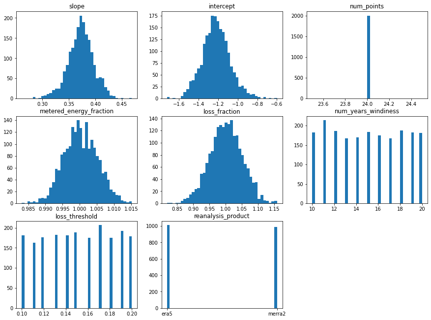
It’s useful to plot distributions of each variable to show what is happening in the Monte Carlo OA method. Based on the plot below, we observe the following:

• metered_energy_fraction, and loss_fraction sampling follow a normal distribution as expected

• The slope and intercept distributions appear normally distributed, even though different reanalysis products are considered, resulting in different regression relationships. This is likely because the reanalysis products agree with each other closely.

• 24 data points were used for all iterations, indicating that there was no variation in the number of outlier months removed

• We see approximately equal sampling of the num_years_windiness, loss_threshold, and reanalysis_product, as expected

plt.figure(figsize=(15,15))
for s in np.arange(mc_reg.shape[1]):
    plt.subplot(4,3,s+1)
    plt.hist(mc_reg.iloc[:,s],40)
    plt.title(mc_reg.columns[s])
plt.show()

It’s worth highlighting the inverse relationship between slope and intercept values under the Monte Carlo approach. Slope and intercept values are strongly negatively correlated (e.g. slope goes up, intercept goes down), as shown below.

# Produce scatter plots of slope and intercept values. Here we focus on the ERA-5 data

plt.figure(figsize=(8,6))
plt.plot(mc_reg.intercept[mc_reg.reanalysis_product =='era5'],mc_reg.slope[mc_reg.reanalysis_product =='era5'],'.')
plt.xlabel('Intercept (GWh)')
plt.ylabel('Slope (GWh / (m/s))')
plt.show()

We can look further at the influence of certain Monte Carlo parameters on the AEP result. For example, let’s see what effect the choice of reanalysis product has on the result:

# Boxplot of AEP based on choice of reanalysis product
tmp_df=pd.DataFrame(data={'aep':pa.results.aep_GWh,'reanalysis_product':mc_reg['reanalysis_product']})
tmp_df.boxplot(column='aep',by='reanalysis_product',figsize=(8,6))
plt.ylabel('AEP (GWh/yr)')
plt.xlabel('Reanalysis product')
plt.title('AEP estimates by reanalysis product')
plt.suptitle("")
plt.show()

In this case, the two reanalysis products lead to similar AEP estimates, although MERRA2 yields slightly higher uncertainty.

We can also look at the effect on the number of years used in the windiness correction:

# Boxplot of AEP based on number of years in windiness correction

tmp_df=pd.DataFrame(data={'aep':pa.results.aep_GWh,'num_years_windiness':mc_reg['num_years_windiness']})
tmp_df.boxplot(column='aep',by='num_years_windiness',figsize=(8,6))
plt.ylabel('AEP (GWh/yr)')
plt.xlabel('Number of years in windiness correction')
plt.title('AEP estimates by windiness years')
plt.suptitle("")
plt.show()

As seen above, the number of years used in the windiness correction does not significantly impact the AEP estimate.

Example operational analysis using the augmented capabilities of the AEP class

%load_ext autoreload
%autoreload 2

This notebook provides an overview and walk-through of the augmented capabilities which have been added to the plant-level operational energy asssessment (OA) of a wind plant in the PRUF project. The La Haute-Borne wind farm is used here and throughout the example notebooks.

The overall structure of the notebook follows the walk-through in the standard AEP example notebook ‘02_plant_aep_analysis,’ to which we refer the reader for a detailed description of the steps needed to prepare the analysis. Here, we focus on the application of various approaches in the AEP calculation, with different time resolutions, regression inputs and regression models used.

import os
import matplotlib.pyplot as plt
import numpy as np
import statsmodels.api as sm
import pandas as pd
import copy

from project_ENGIE import Project_Engie
from operational_analysis.methods import plant_analysis

In the call below, make sure the appropriate path to the CSV input files is specfied. In this example, the CSV files are located directly in the ‘examples/operational_AEP_analysis/data’ folder.

# Load plant object
project = Project_Engie('./data/la_haute_borne')

# Prepare data
project.prepare()

INFO:project_ENGIE:Loading SCADA data
INFO:operational_analysis.types.timeseries_table:Loading name:la-haute-borne-data-2014-2015
INFO:project_ENGIE:SCADA data loaded
INFO:project_ENGIE:Timestamp QC and conversion to UTC
INFO:project_ENGIE:Correcting for out of range of temperature variables
INFO:project_ENGIE:Flagging unresponsive sensors
INFO:project_ENGIE:Converting field names to IEC 61400-25 standard
INFO:operational_analysis.types.timeseries_table:Loading name:plant_data
INFO:operational_analysis.types.timeseries_table:Loading name:plant_data
INFO:operational_analysis.types.timeseries_table:Loading name:merra2_la_haute_borne
INFO:operational_analysis.types.timeseries_table:Loading name:era5_wind_la_haute_borne

Comparison 1: AEP calculation using different regression models and different time resolution

The updated AEP class includes the choice of four different regression algorithms to calculate the long-term OA. The choice is based on what is specified by the reg_model parameter: - linear regression (reg_model = ‘lin’, default) - generalized additive regression model (reg_model = ‘gam’) - gradient boosting regressor (reg_model = ‘gbm’) - extremely randomized trees model (reg_model = ‘etr’)

Linear regression can be selected without restrictions, but should only be used at monthly resolution, since wind plant power curves are not linear at fine time resolution. On the other hand, as machine learning models are more suited for problems with a large number of data points, we have restricted the use of gam, gbm and etr regressors to OA performed at daily and hourly resolution only.

Here, we’ll calculate AEP using all four regression models, using only wind speed as input (Comparison 2 will show an example of a multivariate regression). The linear regression model is run at monthly resolution; the GBM and ETR models at daily resolution; the GAM model at hourly resolution.

pa_lin = plant_analysis.MonteCarloAEP(project, reanal_products = ['merra2','era5'], time_resolution = 'M',
                                    reg_temperature = False, reg_winddirection = False, reg_model = 'lin')

pa_gam = plant_analysis.MonteCarloAEP(project, reanal_products = ['merra2','era5'], time_resolution = 'H',
                                     reg_temperature = False, reg_winddirection = False, reg_model = 'gam')

pa_gbm = plant_analysis.MonteCarloAEP(project, reanal_products = ['merra2','era5'], time_resolution = 'D',
                                         reg_temperature = False, reg_winddirection = False, reg_model = 'gbm')

pa_etr = plant_analysis.MonteCarloAEP(project, reanal_products = ['merra2','era5'], time_resolution = 'D',
                                            reg_temperature = False, reg_winddirection = False, reg_model = 'etr')

INFO:operational_analysis.methods.plant_analysis:Initializing MonteCarloAEP Analysis Object
INFO:operational_analysis.methods.plant_analysis:Initializing MonteCarloAEP Analysis Object
INFO:operational_analysis.methods.plant_analysis:Initializing MonteCarloAEP Analysis Object
INFO:operational_analysis.methods.plant_analysis:Initializing MonteCarloAEP Analysis Object

As an example, the monthly data frame below includes wind speed averages for both the reanalysis products selected for the analysis.

# View the monthly data frame
pa_lin._aggregate.df.head()

	energy_gwh	energy_nan_perc	num_days_expected	num_days_actual	availability_gwh	curtailment_gwh	gross_energy_gwh	availability_pct	curtailment_pct	avail_nan_perc	curt_nan_perc	nan_flag	availability_typical	curtailment_typical	combined_loss_valid	merra2	era5
time
2014-01-01	1.279667	0.0	31	31	0.008721	0.000000	1.288387	0.006769	0.000000	0.0	0.0	False	True	True	True	7.227947	7.314878
2014-02-01	1.793873	0.0	28	28	0.005280	0.000000	1.799153	0.002934	0.000000	0.0	0.0	False	True	True	True	8.598686	8.347006
2014-03-01	0.805549	0.0	31	31	0.000151	0.000000	0.805700	0.000188	0.000000	0.0	0.0	False	True	True	True	5.207071	5.169673
2014-04-01	0.636472	0.0	30	30	0.002773	0.000000	0.639245	0.004338	0.000000	0.0	0.0	False	True	True	True	4.872304	4.756275
2014-05-01	1.154255	0.0	31	31	0.015176	0.000225	1.169656	0.012974	0.000192	0.0	0.0	False	True	True	True	6.351635	6.162751

We now run the Monte-Carlo based OA for the four setups specified above. The following lines of code launch the Monte Carlo-based OA for AEP. We identify each source of uncertainty in the OA estimate and use that uncertainty to create distributions of the input and intermediate variables from which we can sample for each iteration of the OA code.

We repeat the OA process “num_sim” times using different sampling combinations of the input and intermediate variables to produce a distribution of AEP values. Running the OA with the machine learning models at daily resolution is significantly slower than the case of a simple linear regression. Therefore, we have reduced the num_sim parameter to speed up the computation here. Once again, for a detailed description of the steps in the OA process, please refer to the standard AEP example notebook.

# Run Monte-Carlo based OA - linear monthly
pa_lin.run(num_sim=1000)
# Run Monte-Carlo based OA - gam model, hourly resolution
pa_gam.run(num_sim=500)
# Run Monte-Carlo based OA - gradient boosting model, daily resolution
pa_gbm.run(num_sim=500)
# Run Monte-Carlo based OA - extra randomized tree model, daily resolution
pa_etr.run(num_sim=500)

INFO:operational_analysis.methods.plant_analysis:Running with parameters: {'uncertainty_meter': 0.005, 'uncertainty_losses': 0.05, 'uncertainty_loss_max': array([10., 20.]), 'uncertainty_windiness': array([10., 20.]), 'uncertainty_nan_energy': 0.01, 'num_sim': 1000, 'reanal_subset': ['merra2', 'era5']}
100%|██████████| 1000/1000 [00:10<00:00, 93.61it/s]
INFO:operational_analysis.methods.plant_analysis:Run completed
INFO:operational_analysis.methods.plant_analysis:Running with parameters: {'uncertainty_meter': 0.005, 'uncertainty_losses': 0.05, 'uncertainty_loss_max': array([10., 20.]), 'uncertainty_windiness': array([10., 20.]), 'uncertainty_nan_energy': 0.01, 'num_sim': 500, 'reanal_subset': ['merra2', 'era5']}
  0%|          | 0/500 [00:00<?, ?it/s]

Fitting 5 folds for each of 20 candidates, totalling 100 fits

  0%|          | 2/500 [00:09<32:22,  3.90s/it]

Fitting 5 folds for each of 20 candidates, totalling 100 fits

100%|██████████| 500/500 [04:21<00:00,  1.91it/s]
INFO:operational_analysis.methods.plant_analysis:Run completed
INFO:operational_analysis.methods.plant_analysis:Running with parameters: {'uncertainty_meter': 0.005, 'uncertainty_losses': 0.05, 'uncertainty_loss_max': array([10., 20.]), 'uncertainty_windiness': array([10., 20.]), 'uncertainty_nan_energy': 0.01, 'num_sim': 500, 'reanal_subset': ['merra2', 'era5']}
  0%|          | 0/500 [00:00<?, ?it/s]

Fitting 5 folds for each of 20 candidates, totalling 100 fits

  0%|          | 1/500 [00:20<2:52:01, 20.68s/it]

Fitting 5 folds for each of 20 candidates, totalling 100 fits

100%|██████████| 500/500 [02:14<00:00,  3.71it/s]
INFO:operational_analysis.methods.plant_analysis:Run completed
INFO:operational_analysis.methods.plant_analysis:Running with parameters: {'uncertainty_meter': 0.005, 'uncertainty_losses': 0.05, 'uncertainty_loss_max': array([10., 20.]), 'uncertainty_windiness': array([10., 20.]), 'uncertainty_nan_energy': 0.01, 'num_sim': 500, 'reanal_subset': ['merra2', 'era5']}
  0%|          | 0/500 [00:00<?, ?it/s]

Fitting 5 folds for each of 20 candidates, totalling 100 fits

  0%|          | 2/500 [00:30<1:45:54, 12.76s/it]

Fitting 5 folds for each of 20 candidates, totalling 100 fits

100%|██████████| 500/500 [03:32<00:00,  2.35it/s]
INFO:operational_analysis.methods.plant_analysis:Run completed

The key results for the AEP analysis are shown below: distributions of AEP values from which uncertainty can be deduced. We can now compare the AEP distributions obtained for the four configurations of the OA.

# Plot a distribution of AEP values from the Monte-Carlo OA method - wind speed only
pa_lin.plot_result_aep_distributions().show()

# Plot a distribution of AEP values from the Monte-Carlo OA method - gam model
pa_gam.plot_result_aep_distributions().show()

# Plot a distribution of AEP values from the Monte-Carlo OA method - gradient boosting model
pa_gbm.plot_result_aep_distributions().show()

# Plot a distribution of AEP values from the Monte-Carlo OA method - extra randomized tree model
pa_etr.plot_result_aep_distributions().show()

For this specific case, we see a decrease in AEP uncertainty when the calculation is performed with a machine learning regression model at daily resolution, which becomes even more significant when performing the calculation at hourly resolution. Our analysis on a larger set of wind plants (Bodini et al. 2021, Wind Energy) showed how the uncertainty component connected to the regression decreases by up to 60% (relative change) when moving from monthly to daily resolution, and by up to 80% (relative change) when moving from monthly to hourly resolution. Finally, we note how the GBM and ETR regression models are more computationally expensive than the GAM regression model. However, as ensemble-based models, they are expected to be capable of better modeling complex relationships.

Comparison 2: AEP calculation using various input variables

The augmented capabilities of the AEP class now allow the user to include temperature and/or wind direction as additional inputs to the long-term OA. This choice is controlled by the booleans “reg_temperature” and “reg_winddirection”. In this example, we will compute AEP using a multivariate hourly GAM regression, including wind speed and temperature as inputs, and compare the results with the univariate GAM applied in the previous comparison.

pa_gam_T = plant_analysis.MonteCarloAEP(project, reanal_products = ['merra2','era5'], time_resolution = 'H',
                                     reg_temperature = True, reg_winddirection = False, reg_model = 'gam')

INFO:operational_analysis.methods.plant_analysis:Initializing MonteCarloAEP Analysis Object

We now run the Monte-Carlo based OA for this new setup:

# Run Monte-Carlo based OA - gam model
pa_gam_T.run(num_sim=500)

INFO:operational_analysis.methods.plant_analysis:Running with parameters: {'uncertainty_meter': 0.005, 'uncertainty_losses': 0.05, 'uncertainty_loss_max': array([10., 20.]), 'uncertainty_windiness': array([10., 20.]), 'uncertainty_nan_energy': 0.01, 'num_sim': 500, 'reanal_subset': ['merra2', 'era5']}
  0%|          | 0/500 [00:00<?, ?it/s]

Fitting 5 folds for each of 20 candidates, totalling 100 fits

  0%|          | 1/500 [00:17<2:24:14, 17.34s/it]

Fitting 5 folds for each of 20 candidates, totalling 100 fits

100%|██████████| 500/500 [07:23<00:00,  1.13it/s]
INFO:operational_analysis.methods.plant_analysis:Run completed

And we can now take a look at the AEP distribution:

# Plot a distribution of AEP values from the Monte-Carlo OA method - wind speed + temperature + wind direction
pa_gam_T.plot_result_aep_distributions().show()

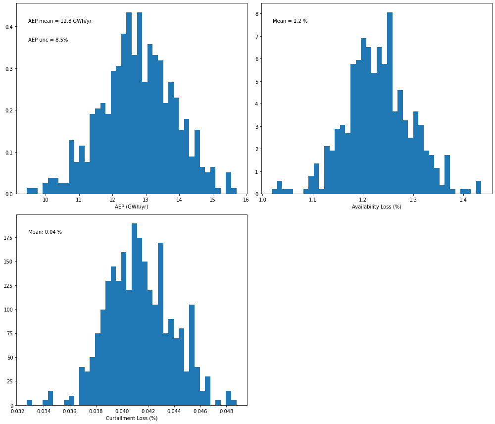
In this case, only a slight reduction in AEP uncertainty is achieved when temperature is added as additional input to the hourly GAM regression. Our analysis (Bodini et al. 2021, Wind Energy) showed how adding temperature as additional input has the largest benefits for those wind plants that experience a strong seasonal cycle, which might not be the case for the specific wind plant considered in this example.

The next step in the gap analysis is to calculate the Turbine Ideal Energy (TIE) for the wind farm based on SCADA data

%load_ext autoreload
%autoreload 2

This notebook provides an overview and walk-through of the turbine ideal energy (TIE) method in OpenOA. The TIE metric is defined as the amount of electricity generated by all turbines at a wind farm operating under normal conditions (i.e., not subject to downtime or significant underperformance, but subject to wake losses and moderate turbine performance losses). The approach to calculate TIE is to:

1. Filter out underperforming data from the power curve for each turbine,

2. Develop a statistical relationship between the remaining power data and key atmospheric variables from a long-term reanalysis product

3. Long-term correct the period of record power data using the above statistical relationship

4. Sum up the long-term corrected power data across all turbines to get TIE for the wind farm

Here we use different reanalysis products to capture the uncertainty around the modeled wind resource. We also consider uncertainty due to power data accuracy and the power curve filtering choices for identifying normal turbine performance made by the analyst.

In this example, the process for estimating TIE is illustrated both with and without uncertainty quantification.

# Import required packages
import matplotlib.pyplot as plt
import numpy as np
import pandas as pd

from project_ENGIE import Project_Engie
from operational_analysis.methods import turbine_long_term_gross_energy

In the call below, make sure the appropriate path to the CSV input files is specfied. In this example, the CSV files are located directly in the ‘examples/data/la_haute_borne’ folder

# Load plant object
project = Project_Engie('./data/la_haute_borne')

# Load and prepare the wind farm data
project.prepare()

INFO:project_ENGIE:Loading SCADA data
INFO:operational_analysis.types.timeseries_table:Loading name:la-haute-borne-data-2014-2015
INFO:project_ENGIE:SCADA data loaded
INFO:project_ENGIE:Timestamp QC and conversion to UTC
INFO:project_ENGIE:Correcting for out of range of temperature variables
INFO:project_ENGIE:Flagging unresponsive sensors
INFO:project_ENGIE:Converting field names to IEC 61400-25 standard
INFO:operational_analysis.types.timeseries_table:Loading name:plant_data
INFO:operational_analysis.types.timeseries_table:Loading name:plant_data
INFO:operational_analysis.types.timeseries_table:Loading name:merra2_la_haute_borne
INFO:operational_analysis.types.timeseries_table:Loading name:era5_wind_la_haute_borne

# Let's take a look at the columns in the SCADA data frame
project._scada.df.columns

Index(['id', 'wrot_BlPthAngVal1_avg', 'wmet_wdspd_avg', 'wmet_VaneDir_avg',
       'wmet_EnvTmp_avg', 'wyaw_YwAng_avg', 'wmet_HorWdDir_avg', 'wtur_W_avg',
       'energy_kwh'],
      dtype='object')

TIE calculation without uncertainty quantification

Next we create a TIE object which will contain the analysis to be performed. The method has the ability to calculate uncertainty in the TIE metric through a Monte Carlo sampling of filtering thresholds, power data, and reanalysis product choices. For now, we turn this option off and run the method a single time.

ta = turbine_long_term_gross_energy.TurbineLongTermGrossEnergy(project, UQ=False)

INFO:operational_analysis.methods.turbine_long_term_gross_energy:Initializing TurbineLongTermGrossEnergy Object
INFO:operational_analysis.methods.turbine_long_term_gross_energy:Note: uncertainty quantification will NOT be performed in the calculation
INFO:operational_analysis.methods.turbine_long_term_gross_energy:Processing SCADA data into dictionaries by turbine (this can take a while)

All of the steps in the TI calculation process are pulled under a single run() function. These steps include:

1. Processing reanalysis data to daily averages.

2. Filtering the SCADA data

3. Fitting the daily reanalysis data to daily SCADA data using a Generalized Additive Model (GAM)

4. Apply GAM results to calculate long-term TIE for the wind farm

By setting UQ = False (the default argument value), we must manually specify key filtering thresholds that would otherwise be sampled from a range of values through Monte Carlo. Specifically, we must set thresholds applied to the bin_filter() function in the toolkits.filtering class of OpenOA.

# Specify filter threshold values to be used
wind_bin_thresh = 2.0 # Exclude data outside 2 standard deviations of the median for each power bin
max_power_filter = 0.90 # Don't apply bin filter above 0.9 of turbine capacity

We also must decide how to deal with missing data when computing daily sums of energy production from each turbine. Here we set the threshold at 0.9 (i.e., if greater than 90% of SCADA data are available for a given day, scale up the daily energy by the fraction of data missing. If less than 90% data recovery, exclude that day from analysis.

# Set the correction threshold to 90%
correction_threshold = 0.90

Now we’ll call the run() method to calculate TIE, choosing two reanalysis products to be used in the TIE calculation process.

# We can choose to save key plots to a file by setting enable_plotting = True and
# specifying a directory to save the images. For now we turn off this feature.
ta.run(reanal_subset = ['era5', 'merra2'], enable_plotting = False, plot_dir = None,
       wind_bin_thresh = wind_bin_thresh, max_power_filter = max_power_filter,
       correction_threshold = correction_threshold)

  0%|          | 0/2 [00:00<?, ?it/s]INFO:operational_analysis.methods.turbine_long_term_gross_energy:Filtering turbine data
INFO:operational_analysis.methods.turbine_long_term_gross_energy:Processing reanalysis data to daily averages
INFO:operational_analysis.methods.turbine_long_term_gross_energy:Processing scada data to daily sums

4it [00:00, 42.75it/s]
INFO:operational_analysis.methods.turbine_long_term_gross_energy:Setting up daily data for model fitting
INFO:operational_analysis.methods.turbine_long_term_gross_energy:Fitting model data
INFO:operational_analysis.methods.turbine_long_term_gross_energy:Applying fitting results to calculate long-term gross energy
 50%|█████     | 1/2 [00:01<00:01,  1.20s/it]INFO:operational_analysis.methods.turbine_long_term_gross_energy:Filtering turbine data
INFO:operational_analysis.methods.turbine_long_term_gross_energy:Processing reanalysis data to daily averages
INFO:operational_analysis.methods.turbine_long_term_gross_energy:Processing scada data to daily sums

0it [00:00, ?it/s]
4it [00:00, 35.64it/s]
INFO:operational_analysis.methods.turbine_long_term_gross_energy:Setting up daily data for model fitting
INFO:operational_analysis.methods.turbine_long_term_gross_energy:Fitting model data
INFO:operational_analysis.methods.turbine_long_term_gross_energy:Applying fitting results to calculate long-term gross energy
100%|██████████| 2/2 [00:02<00:00,  1.20s/it]
INFO:operational_analysis.methods.turbine_long_term_gross_energy:Run completed

Now that we’ve finished the TIE calculation, let’s examine results

ta._plant_gross

array([[13536202.10370381],
       [13644554.87775164]])

# What is the long-term annual TIE for whole plant
print('Long-term turbine ideal energy is %s GWh/year' %np.round(np.mean(ta._plant_gross/1e6),1))

Long-term turbine ideal energy is 13.6 GWh/year

The long-term TIE value of 13.6 GWh/year is based on the mean TIE resulting from the two reanalysis products considered.

Next, we can examine how well the filtering worked by examining the power curves for each turbine using the plot_filtered_power_curves() function.

# Currently saving figures in examples folder. The folder where figures are saved can be changed if desired.
ta.plot_filtered_power_curves(save_folder = "./", output_to_terminal = True)

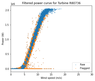
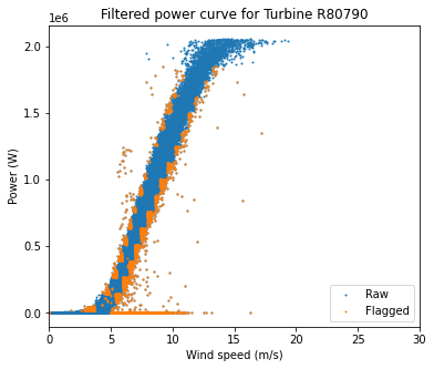
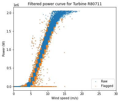
Overall these are very clean power curves, and the filtering algorithms seem to have done a good job of catching the most egregious outliers.

Now let’s look at the daily data and how well the power curve fit worked

# Currently saving figures in examples folder. The folder where figures are saved can be changed if desired.
ta.plot_daily_fitting_result(save_folder = "./", output_to_terminal = True)

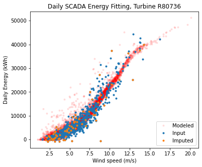
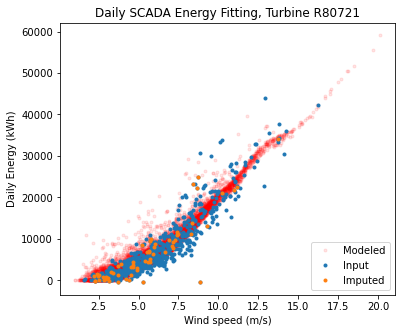
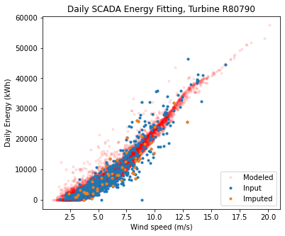
Overall the fit looks good. The modeled data sometimes estimate higher energy at low wind speeds compared to the observed, but keep in mind the model fits to long term wind speed, wind direction, and air density, whereas we are only showing the relationship to wind speed here.

Note that ‘imputed’ means daily power data that were missing for a specific turbine, but were calculated by establishing statistical relationships with that turbine and its neighbors. This is necessary since a wind farm often has one turbine down and, without imputation, very little daily data would be left if we excluded days when a turbine was down.

TIE calculation including uncertainty quantification

Now we will create a TIE object for calculating TIE and quantifying the uncertainty in our estimate. The method estimates uncertainty in the TIE metric through a Monte Carlo sampling of filtering thresholds, power data, and reanalysis product choices.

Note that we set the number of Monte Carlo simulations to only 100 in this example because of the relatively high computational effort required to perform a single iteration. In practice, a larger number of simulations is recommended (the default value is 2000).

ta = turbine_long_term_gross_energy.TurbineLongTermGrossEnergy(project,
                                                               UQ = True, # enable uncertainty quantification
                                                               num_sim = 100 # number of Monte Carlo simulations to perform
                                                              )

INFO:operational_analysis.methods.turbine_long_term_gross_energy:Initializing TurbineLongTermGrossEnergy Object
INFO:operational_analysis.methods.turbine_long_term_gross_energy:Note: uncertainty quantification will be performed in the calculation
INFO:operational_analysis.methods.turbine_long_term_gross_energy:Processing SCADA data into dictionaries by turbine (this can take a while)

With uncertainty quantification enabled (UQ = True), we can specify the assumed uncertainty of the SCADA power data (0.5% by default) and ranges of two key filtering thresholds from which the Monte Carlo simulations will sample. Specifically, these thresholds are applied to the bin_filter() function in the toolkits.filtering class of OpenOA.

Note that the following parameters are the default values used in the run() method.

uncertainty_scada=0.005 # Assumed uncertainty of SCADA power data (0.5%)

# Range of filter threshold values to be used by Monte Carlo simulations

# Data outside of a range of +-1 to +-3 standard deviations from the median for each power bin are discarded
wind_bin_thresh=(1, 3)

# The bin filter will be applied up to fractions of turbine capacity from 80% to 90%
max_power_filter=(0.8, 0.9)

We will consider a range of availability thresholds for dealing with missing data when computing daily sums of energy production from each turbine (i.e., if greater than the given threshold of SCADA data are available for a given day, scale up the daily energy by the fraction of data missing. If less than the given threshold of data are available, exclude that day from analysis. Here we set the range of thresholds as 85% to 95%.

correction_threshold=(0.85, 0.95)

Now we’ll call the run() method to calculate TIE with uncertainty quantification, again choosing two reanalysis products to be used in the TIE calculation process.

Note that without uncertainty quantification (UQ = False), a separate TIE value is calculated for each reanalysis product specified. However, when UQ = True, the reanalysis product is treated as another Monte Carlo sampling parameter. Thus, the impact of different reanlysis products is considered to be part of the overall uncertainty in TIE.

# We can choose to save key plots to a file by setting enable_plotting = True and
# specifying a directory to save the images. For now we turn off this feature.
ta.run(reanal_subset = ['era5', 'merra2'], enable_plotting = False, plot_dir = None,
       uncertainty_scada = uncertainty_scada, wind_bin_thresh = wind_bin_thresh,
       max_power_filter = max_power_filter, correction_threshold = correction_threshold)

Now that we’ve finished the Monte Carlo TIE calculation simulations, let’s examine results

np.mean(ta._plant_gross)

13523325.942440799

np.std(ta._plant_gross)

316720.1040105598

# Mean long-term annual TIE for whole plant
print('Mean long-term turbine ideal energy is %s GWh/year' %np.round(np.mean(ta._plant_gross/1e6),1))

# Uncertainty in long-term annual TIE for whole plant
print('Uncertainty in long-term turbine ideal energy is %s GWh/year, or %s percent' % (np.round(np.std(ta._plant_gross/1e6),1), np.round(100*np.std(ta._plant_gross)/np.mean(ta._plant_gross),1)))

Mean long-term turbine ideal energy is 13.5 GWh/year
Uncertainty in long-term turbine ideal energy is 0.3 GWh/year, or 2.3 percent

As expected, the mean long-term TIE is close to the earlier estimate without uncertainty quantification. A relatively low uncertainty has been estimated for the TIE calculations. This is a result of the relatively close agreement between the two reanalysis products and the clean power curves plotted earlier.

The next step in the gap analysis is to estimate electrical losses from the wind farm.

%load_ext autoreload
%autoreload 2

Calculating electrical losses in this method is relatively straightforward. In short, the sum of turbine energy is compared to the sum of metered energy, with the differnce equaling the electrical losses for the wind farm. However, the time resolution of the metered data and dealing with missing data are important aspects of this method.

The approach is to first calculate daily sums of turbine and revenue meter energy over the plant period of record. Only those days where all turbines and the revenue meter were reporting for all timesteps are considered. Electrical loss is then the difference in total turbine energy production and meter production over those concurrent days.

Uncertainty in the calculated electrical losses is estimated by applying a Monte Carlo approach to sample revenue meter data and SCADA data with a 0.5% imposed uncertainty. One filtering parameter is sampled too. The uncertainty in estimated electrical losses is quantified as the standard deviation of the distribution of losses obtained from the MC sampling.

In this example, the procedure for calculating electrical losses is illustrated with and without uncertainty quantification.

In the case that meter data is not provided on a daily or sub-daily basis (e.g. monthly), a different approach is implemented. The sum of daily turbine energy is corrected for any missing reported energy data from the turbines based on the ratio of expected number of data counts per day to the actual. Daily corrected sum of turbine energy is then summed on a monthly basis. Electrical loss is then the difference between total corrected turbine energy production and meter production over those concurrent months.

# Import required packages
import matplotlib.pyplot as plt
import numpy as np
import pandas as pd

from project_ENGIE import Project_Engie
from operational_analysis.methods import electrical_losses

In the call below, make sure the appropriate path to the CSV input files is specfied. In this example, the CSV files are located directly in the ‘examples/operational_AEP_analysis/data’ folder.

# Load wind farm object
project = Project_Engie('./data/la_haute_borne')

# Load and prepare the wind farm data
project.prepare()

INFO:project_ENGIE:Loading SCADA data
INFO:operational_analysis.types.timeseries_table:Loading name:la-haute-borne-data-2014-2015
INFO:project_ENGIE:SCADA data loaded
INFO:project_ENGIE:Timestamp QC and conversion to UTC
INFO:project_ENGIE:Correcting for out of range of temperature variables
INFO:project_ENGIE:Flagging unresponsive sensors
INFO:numexpr.utils:NumExpr defaulting to 8 threads.
INFO:project_ENGIE:Converting field names to IEC 61400-25 standard
INFO:operational_analysis.types.timeseries_table:Loading name:plant_data
INFO:operational_analysis.types.timeseries_table:Loading name:plant_data
INFO:operational_analysis.types.timeseries_table:Loading name:merra2_la_haute_borne
INFO:operational_analysis.types.timeseries_table:Loading name:era5_wind_la_haute_borne

Electrical loss estimation without uncertainty quantification

Next we create an Electrical Loss object which will contain the analysis to be performed. The method has the ability to calculate uncertainty in the electrical losses through a Monte Carlo sampling of power data based on its measurement uncertainty. For now, we turn this option off and calculate a single electrical loss value.

# Create Electrical Loss object
el = electrical_losses.ElectricalLosses(project)

INFO:operational_analysis.methods.electrical_losses:Initializing Electrical Losses Object
INFO:operational_analysis.methods.electrical_losses:Note: uncertainty quantification will NOT be performed in the calculation

# Now we run the analysis using the run() function in the method
el.run(uncertainty_correction_thresh=0.95 # If dealing with monthly meter data, exclude months with less than 95%
                                          # data coverage
      )

INFO:operational_analysis.methods.electrical_losses:Processing SCADA data
INFO:operational_analysis.methods.electrical_losses:Processing meter data
INFO:operational_analysis.methods.electrical_losses:Calculating electrical losses
100%|██████████| 1/1 [00:00<00:00, 123.34it/s]

Now that the analyiss is complete, let’s examine the results

el._electrical_losses[0][0]

0.019994645742959616

# Electrical losses for the wind farm
print('Electrical losses are %s percent' % np.round(el._electrical_losses[0][0]*100,1))

Electrical losses are 2.0 percent

Now let’s plot electrical losses by month

plt.figure(figsize = (8,4))
monthly_merge = el._merge_df.resample('MS').sum()
plt.plot((monthly_merge['corrected_energy'] - monthly_merge['energy_kwh']) / monthly_merge['corrected_energy'] * 100)
plt.xlabel('Month')
plt.ylabel('Electrical Losses (%)')

/Users/esimley/opt/anaconda3/lib/python3.7/site-packages/pandas/plotting/_converter.py:129: FutureWarning: Using an implicitly registered datetime converter for a matplotlib plotting method. The converter was registered by pandas on import. Future versions of pandas will require you to explicitly register matplotlib converters.

To register the converters:
        >>> from pandas.plotting import register_matplotlib_converters
        >>> register_matplotlib_converters()
  warnings.warn(msg, FutureWarning)

Text(0, 0.5, 'Electrical Losses (%)')

We see that electrical losses vary between 1.98 and 2.02%. This is a narrow range, but keep in mind the meter data for La Haute Borne was synthesized by NREL based on the SCADA data and sampling around a 2% electrical loss with a standard deviation of 0.5%. Part of the reason for the very low spread in estimated monthly electrical losses is that uncertainty was introduced to the meter data at the 10-minute level when the data were synthesized. This uncertainty tends to get averaged out over the period of record. Normally electrical losses using actual meter data would not be this consistent and would generally show seasonal trends.

Electrical loss estimation including uncertainty quantification

Next we create an Electrical Loss object with uncertainty quantification enabled and the number of Monte Carlo simulations set to 3000. This method calculates uncertainty in the electrical losses through a Monte Carlo sampling of power data based on its assumed measurement uncertainty of 0.5%. Furthermore, if dealing with monthly meter data, a range of availabiity thresholds used to remove months with low data coverage is sampled.

# Create Electrical Loss object
el = electrical_losses.ElectricalLosses(project, UQ = True, # enable UQ
                                        num_sim = 3000 # number of Monte Carlo simulations to perform
                                       )

INFO:operational_analysis.methods.electrical_losses:Initializing Electrical Losses Object
INFO:operational_analysis.methods.electrical_losses:Note: uncertainty quantification will be performed in the calculation

# Now we run the analysis using the run() function in the method
el.run(uncertainty_meter=0.005, # 0.5% uncertainty in meter data
       uncertainty_scada=0.005, # 0.5% uncertainty in scada data
       uncertainty_correction_thresh=(0.9, 0.995) # If dealing with monthly meter data, exclude months with less than 95%
                                          # data coverage
      )

INFO:operational_analysis.methods.electrical_losses:Processing SCADA data
INFO:operational_analysis.methods.electrical_losses:Processing meter data
INFO:operational_analysis.methods.electrical_losses:Calculating electrical losses
100%|██████████| 3000/3000 [00:10<00:00, 292.52it/s]

Now let’s examine the results from the Monte Carlo simulations

np.mean(el._electrical_losses)

0.02008757941003309

np.std(el._electrical_losses)

0.006770014201072663

# Electrical losses for the wind farm
print('Electrical losses are %s percent' % np.round(np.mean(el._electrical_losses)*100,1))

print('Uncertainty in the electrical loss estimate is %s percent' % np.round(np.std(el._electrical_losses)*100,1))

Electrical losses are 2.0 percent
Uncertainty in the electrical loss estimate is 0.7 percent

Again, the expected electrical losses are 2.0 percent. The uncertainty in the calculated losses is estimated to be 0.7%. This uncertainty value is given by the standard deviation of electrical losses over all Monte Carlo iterations and is primarily driven by the assumed 0.5% uncertainty for meter and SCADA power values.

Perform energy yield assessment (EYA)-operational assessment (OA) gap analysis

This notebook will explore the use of the energy yield assessment (EYA) gap analysis method in OpenOA. This method attributes differences in an EYA-estimate and an operational assessment (OA) estimate of annual energy production (AEP; or net energy, P50). Differences in availability loss estimates, electrical loss estimates, and turbine ideal energy estimates are analyzed. The latter metric incorporates many aspects of an EYA, including the wind resource estimate, wake loss estimate, turbine performance, and blade degradation.

The gap analysis is based on comparing the following three key metrics:

1. Availability loss

2. Electrical loss

3. Sum of turbine ideal energy

Here turbine ideal energy is defined as the energy produced during ‘normal’ or ‘ideal’ turbine operation, i.e., no downtime or considerable underperformance events. This value encompasses several different aspects of an EYA (wind resource estimate, wake losses, turbine performance, and blade degradation) and in most cases should have the largest impact in a gap analysis relative to the first two metrics.

This gap analysis method is fairly straighforward. Relevant EYA and OA metrics are passed in when defining the class, differences in EYA estimates and OA results are calculated, and then a ‘waterfall’ plot is created showing the differences between the EYA and OA-estimated AEP values and how they are linked from differences in the three key metrics.

Waterfall plot code was taken and modified from the following post: https://pbpython.com/waterfall-chart.html

# Import required packages
from project_ENGIE import Project_Engie
from operational_analysis.methods import plant_analysis
from operational_analysis.methods import turbine_long_term_gross_energy
from operational_analysis.methods import electrical_losses
from operational_analysis.methods import eya_gap_analysis

/Users/esimley/opt/anaconda3/lib/python3.7/site-packages/statsmodels/tools/_testing.py:19: FutureWarning: pandas.util.testing is deprecated. Use the functions in the public API at pandas.testing instead.
  import pandas.util.testing as tm

# Load plant object and process plant data
project = Project_Engie('./data/la_haute_borne')
project.prepare()

INFO:project_ENGIE:Loading SCADA data
INFO:operational_analysis.types.timeseries_table:Loading name:la-haute-borne-data-2014-2015
INFO:project_ENGIE:SCADA data loaded
INFO:project_ENGIE:Timestamp QC and conversion to UTC
INFO:project_ENGIE:Correcting for out of range of temperature variables
INFO:numexpr.utils:NumExpr defaulting to 8 threads.
INFO:project_ENGIE:Flagging unresponsive sensors
INFO:project_ENGIE:Converting field names to IEC 61400-25 standard
INFO:operational_analysis.types.timeseries_table:Loading name:plant_data
INFO:operational_analysis.types.timeseries_table:Loading name:plant_data
INFO:operational_analysis.types.timeseries_table:Loading name:merra2_la_haute_borne
INFO:operational_analysis.types.timeseries_table:Loading name:era5_wind_la_haute_borne

Calculate AEP, TIE, and electrical losses from operational data

The first step is to calculate annual energy production (AEP) for the wind farm (Example 02), turbine ideal energy (TIE) for the wind farm (Example 03) and calculate electrical losses (Example 04). Please refer to detailed documentation of these methods in the previous example notebooks.

# Calculate AEP
pa = plant_analysis.MonteCarloAEP(project, reanal_products = ['era5', 'merra2'])
pa.run(num_sim=20000, reanal_subset=['era5', 'merra2'])

INFO:operational_analysis.methods.plant_analysis:Initializing MonteCarloAEP Analysis Object
INFO:operational_analysis.methods.plant_analysis:Running with parameters: {'uncertainty_meter': 0.005, 'uncertainty_losses': 0.05, 'uncertainty_loss_max': array([10., 20.]), 'uncertainty_windiness': array([10., 20.]), 'uncertainty_nan_energy': 0.01, 'num_sim': 20000, 'reanal_subset': ['era5', 'merra2']}
100%|██████████| 20000/20000 [05:14<00:00, 63.62it/s]
INFO:operational_analysis.methods.plant_analysis:Run completed

# Calculate TIE
ta = turbine_long_term_gross_energy.TurbineLongTermGrossEnergy(project, UQ=False)
ta.run(reanal_subset = ['era5', 'merra2'],
       max_power_filter = 0.85,
       wind_bin_thresh = 2.0,
       correction_threshold = 0.90,
       enable_plotting = False,
       plot_dir = None)

INFO:operational_analysis.methods.turbine_long_term_gross_energy:Initializing TurbineLongTermGrossEnergy Object
INFO:operational_analysis.methods.turbine_long_term_gross_energy:Note: uncertainty quantification will NOT be performed in the calculation
INFO:operational_analysis.methods.turbine_long_term_gross_energy:Processing SCADA data into dictionaries by turbine (this can take a while)
  0%|          | 0/2 [00:00<?, ?it/s]INFO:operational_analysis.methods.turbine_long_term_gross_energy:Filtering turbine data
INFO:operational_analysis.methods.turbine_long_term_gross_energy:Processing reanalysis data to daily averages
INFO:operational_analysis.methods.turbine_long_term_gross_energy:Processing scada data to daily sums

0it [00:00, ?it/s]
4it [00:00, 23.20it/s]
INFO:operational_analysis.methods.turbine_long_term_gross_energy:Setting up daily data for model fitting
INFO:operational_analysis.methods.turbine_long_term_gross_energy:Fitting model data
INFO:operational_analysis.methods.turbine_long_term_gross_energy:Applying fitting results to calculate long-term gross energy
 50%|█████     | 1/2 [00:02<00:02,  2.46s/it]INFO:operational_analysis.methods.turbine_long_term_gross_energy:Filtering turbine data
INFO:operational_analysis.methods.turbine_long_term_gross_energy:Processing reanalysis data to daily averages
INFO:operational_analysis.methods.turbine_long_term_gross_energy:Processing scada data to daily sums

0it [00:00, ?it/s]
4it [00:00, 21.38it/s]
INFO:operational_analysis.methods.turbine_long_term_gross_energy:Setting up daily data for model fitting
INFO:operational_analysis.methods.turbine_long_term_gross_energy:Fitting model data
INFO:operational_analysis.methods.turbine_long_term_gross_energy:Applying fitting results to calculate long-term gross energy
100%|██████████| 2/2 [00:04<00:00,  2.49s/it]
INFO:operational_analysis.methods.turbine_long_term_gross_energy:Run completed

# Calculate electrical losses
el = electrical_losses.ElectricalLosses(project)
el.run()

INFO:operational_analysis.methods.electrical_losses:Initializing Electrical Losses Object
INFO:operational_analysis.methods.electrical_losses:Note: uncertainty quantification will NOT be performed in the calculation
INFO:operational_analysis.methods.electrical_losses:Processing SCADA data
INFO:operational_analysis.methods.electrical_losses:Processing meter data
INFO:operational_analysis.methods.electrical_losses:Calculating electrical losses
100%|██████████| 1/1 [00:00<00:00, 85.36it/s]

Now that we’ve calculated the key operational metrics, we setup some arrays that the gap analysis method needs to run.

Summarize operational results and create EYA data for comparison

# First summarize key operational results
aep = pa.results.aep_GWh.mean()
avail = pa.results.avail_pct.mean()
elec = el._electrical_losses[0][0]
tie = ta._plant_gross[0][0]/1e6

print(aep, avail, elec, tie)

12.289504915814765 0.011694303107633754 0.019994645742960393 13.542669137731398

# Define operational data list
oa_list = [aep, avail, elec, tie]
# AEP (GWh/yr), availability loss (fraction), electrical loss (fraction), turbine ideal energy (GWh/yr)

# Define EYA data list (we are fabricating these values here as an example)
eya_list = [16.46, 20., 0.04, 0.014, 0.037, 0.011, 0.087]
# AEP (GWh/yr), Gross energy (GWh/yr), availability loss (fraction), electrical loss (fraction), turbine performance loss (fraction)
# blade degradation loss (fraction), wake loss (fraction)

Perform gap analysis

Now that we have the data we need, we first create a gap analysis object

gap_anal = eya_gap_analysis.EYAGapAnalysis(plant = 'La Haute Borne', eya_estimates = eya_list, oa_results = oa_list)

INFO:operational_analysis.methods.eya_gap_analysis:Initializing EYA Gap Analysis Object

Now we run the analysis, which by default outputs a waterfall plot showing how the gap between EYA-reported AEP and plant-measured AEP can be explained:

gap_anal.run()

INFO:operational_analysis.methods.eya_gap_analysis:Gap analysis complete

In this example, they EYA estimate of AEP was about 4 GWh/yr higher than the OA result. This difference is largely explained by a large difference in turbine ideal energy (overestimated in EYA), and smaller differences in availability (underestimated in EYA) and electrical losses (overestimated in EYA). A total of 1 GWh/yr is left unexplained or uncertain using this method.